


 nova página do texto(beta)
 Inglês (pdf)
 Artigo em XML
 Referências do artigo
 Enviar este artigo por email
 Citado por SciELO
  Similares em
SciELO
Similares em
SciELO 
 Permalink
1. Introduction
Science interest in synchronization dates back to the late 17th century, when Christiaan Huygens discovered this phenomenon. By the end of the last century a solid mathematical theory was developed, and for the first time it allowed us to really understand some of the simplest examples of synchronization 1-3. However, the general problem is open for research, and the behavior of some apparently simple systems reveals unanswered questions that still need to be answered- see for instance 4, Chapter 8.
By definition, an oscillator has closed phase-space trajectories. In the case of nonlinear oscillators, these closed trajectories may correspond to nonlocal stable regions or attractors, also known as stable limit cycles. According to their limit cycle speed, nonlinear oscillators can be classified into what we call quasi-harmonic and relaxation oscillators. In a quasiharmonic oscillator the trajectory speed along the limit cycle varies smoothly. Contrarily, the speed in a relaxation oscillator presents abrupt changes, thus defining multiple times scales.
Much of the work on synchronization, and concomitantly many of the existing developments, correspond to quasiharmonic oscillators 1,5-7. Regarding relaxation oscillators, their synchronization has been widely studied when they are pulse-coupled-i.e. when the interaction occurs only during the rapid cycle phases 2,3,7-17. This includes:
Master-slave and mutual interaction scenarios.
Two interacting oscillators and large networks of interacting oscillators.
Theoretical and experimental studies.
Contrarily to pulse coupling, in the so-called diffusivelycoupled relaxation oscillators, interaction occurs during the whole cycle. Studying synchronization with this type of interaction is challenging because of the existence of very different times scales. To the best of our knowledge, there is no general mathematical theory for this problem. However, important developments have been achieved while studying specific examples 18-21. On the other hand, only a few experimental studies concerning synchronization of diffusively coupled relaxation oscillators have been reported 22. In this regard, recent developments in electronics, like new digital devices and versatile micro-controllers, make possible the implementation of experimental setups to thoroughly study assemblies of coupled electronic oscillators. Having this in mind, the present work is advocated to experimentally and theoretically studying the synchronization dynamics of two diffusively-coupled electronic relaxation oscillators (based in the 555 integrated circuit, operating in astable mode).
2. Circuit design
2.1. The 555 timer IC
The 555 timer is a very versatile integrated circuit that is frequently used in a variety of timer, pulse generation, and oscillator applications. The detailed characteristics and modes of operation of this circuit can be consulted in 23. In summary, the 555 IC has eight pins that are connected and/or have the functions described as follows:
Pin 1 is connected to the ground reference, or low level voltage (0 V).
Pin 2 is an input pin called the trigger. The output pin goes high when this input falls below 1/2 of the control voltage, which is typically 2/3 of the positive supply voltage, Vs. That is, the output pin goes usually high when voltage at Pin 2 falls bellow 1/3 of Vs.
Pin 3 is the 555 IC output pin. Its voltage can be equal to either Vs or 0 V, depending on the state of the trigger, reset, and threshold pins.
Pin 4 is the reset pin. Voltage at this input needs to be higher than about 1 V in order for Pins 3 and 7 to be able to switch between their available states.
Pin 5 is an input pin that provides access to the control voltage. If this pin is unconnected, the control voltage takes its default value: 2/3 Vs. Usually this function is not required and the control input is often left unconnected.
Pin 6 is an input pin known as the threshold pin. Voltage at the output pin goes low when the voltage at this pin is greater than the control voltage (2/3 Vs if pin 5 unconnected).
Pin 7 is called the discharge pin. It is an open collector output which may discharge a capacitor in phase with the output pin.
Pin 8 is the power input pin. It must be connected to the positive supply voltage (Vs), which provides the power necessary for the IC to operate.
2.2. Electronic oscillator based on the 555 integrated-circuit operating in astable mode
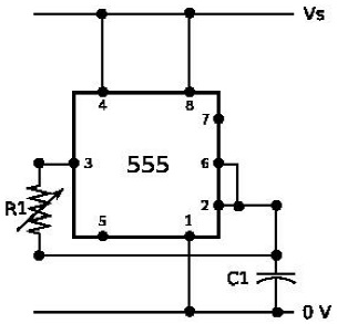
Depending on the way it is connected, the 555 timer IC has two different modes of operation: monostable and astable- see Ref. 23, Sec. 7.4. In the monostable mode, the timer functions as a device that generates a single voltage pulse (of fixed duration) at Pin 3, in response to a negative trigger pulse of less than 1/3 Vs to Pin 2. In the present work we do not employ this configuration, but that corresponding to the astable mode, in which the 555 Timer IC triggers itself and free run as an oscillator-see Fig. 1. According to the description in the previous subsection, the circuit oscillatory behavior can be explained as follows. Assume that capacitor C1 is initially discharged and that the voltage at pin 3 is high. Then, the capacitor starts charging through resistor R1. When the voltage in the upper end of C1 exceeds 2/3 Vs, the voltage at pin 3 shifts to low. This makes the capacitor discharge through resistor R1, until the voltage at the C1 upper end goes below 1/3 Vs. At this point, the voltage at pin 3 changes to high and the cycle starts all over again. Notice that capacitor C1 charges and discharges through R1, producing symmetric cycles. Henceforth, by varying the value of this resistor one can control the cycle period.
2.3. Two mutually interacting 555-IC electronic oscillators
We are interested in studying the synchronization dynamics of two mutually interacting 555-IC electronic oscillators. To do this, we implemented the circuit schematically represented in Fig. 2. Notice that Pins 2-6 in the ICs of both electronic oscillators are connected through a resistor Rc. The rational for this design is that when Rc tends to infinity, the two oscillators behave independently. However, at low resistance values, any voltage difference between the upper ends of Capacitors C1 and C2 would rapidly tend to disappear due to the current the voltage difference causes through resistor Rc, and this in turn may force the oscillators to synchronize. In the experimental protocol described below, we keep fixed the the natural frequency of one oscillator, and variate the frequency of the other. Without loss of generality, we call the oscillator with variable frequency Oscillator 1, and refer to the other as Oscillator 2. The frequency of Oscillator 1 is controlled by modifying resistance R1.
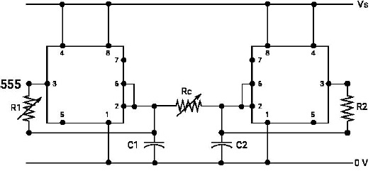
The values of all the resistances and capacitances employed in our circuit design, as well as that of Vs, are tabulated in Table I. Notice that resistance R2, which determines the natural frequency of Oscillator 2, is fixed. With the parameters in I, this frequency should be about 10.5 kHz, but the actual value in a given circuit may change due to electronic-component variability.
Table I Parameter values for the circuit in Fig. 2.
| Parameter | Value | Parameter | Value |
|---|---|---|---|
| R1 | 0-10.0 kΩ | C1 | .01 μF |
| R2 | 6.8kΩ | C2 | 0.01μF |
| Rc | 0-10.0 kΩ | Vs | 5.0V |
3. Data acquisition and experimental results
Data, in the form of voltage time series measured at Pin 3 of both 555 ICs (see Fig. 2) were acquired by means of a BitScope BS10 (manufactured by BitScope 24), controlled from Python 2.7 via the public library BitScope Library 2.0. We used a sampling frequency of 1,000 kHz, and obtained 6,000 data points each time we recorded. This ensures that about 100 data points are captured per cycle, and that more than 50 cycles are recorded each time. We carried out measurements with several combinations of resistances R1 and Rc in the range [0kΩ,10kΩ]. To that end, we employed Dallas Semiconductors’ DS1083 integrated circuit, that features two independently controlled 256-position potentiometers. Control of this device from Python 2.7 was achieved by means of Adafruit FT232H breakout, together with Adafruit Python GPIO library.
Using the above described experimental setup, we recorded data for several values of resistances R1 and Rc (including the case in which both oscillators are uncoupled: Rc → ∞). In Fig. 3, we show sample recordings in which R1=5.85kΩ, and either Rc→∞, or Rc=1.95kΩ. Notice how in the first case both oscillators have different frequencies and so they are out of synchrony, while in the second case not only they are synchronized but they are in phase.

Figure 3 Sample recordings from Pin 3 (V3) of oscillators 1 (orange line) and 2 (blue line). In the corresponding experimental setup, R1 was set to 5.85 kΩ. In the top plot, both oscillators are uncoupled, while in the bottom plot the coupling resistance, Rc, was set to 1.95 kΩ.
To further validate the circuit performance, we carried out recordings for several values of R1 in the range [2.5 kΩ, 10.0 kΩ, while both oscillators are uncoupled (Rc → ∞). Resistance R1 was fixed to 6.8 kΩ. There after, we measured the cycling frequency of Oscillators

Figure 4 Cycling frequency of Oscillator 1 (
To investigate the effects upon synchronization of the coupling resistance value and of the oscillators’ naturalfrequency difference, we performed recordings of the voltage at Pin 3 of both 555 ICs for many different values of resistances R1 and Rc. To test for bistability, we repeated the experiment four different times. In each experiment, one resistance value was fixed while the other was modified stepwise within the corresponding range. Then, the first resistance value was slightly modified, and the whole process was iteratively repeated for a given range of the first resistance values. What changed in each experiment were the initial values of both resistances. Specifically, we selected all possible combinations of the maximum and minimum R1 and Rc values.
After carrying out the above described recordings and plotting the time-series we obtained
from both oscillators, we noticed that the coupled system achieved in general
complex m : n phase-locking rhythms-see 25 Chapter 6. In these, the behavior of the
coupled system is periodically repeated. However, in every period of the coupled
system, each individual oscillator undergoes a different number of cycles. To
characterize these complex rhythms, we measured the frequency of both electronic
oscillators by means of Numpy’s rfft algorithm (let f
1
and f
2
respectively denote the frequencies of Oscillators 1 and 2). Then, we
looked for the greatest common divisor of
f1 and
f2
(gcd(f1
,f2)), and reported rotation number
of the corresponding complex rhythm as m : n, with
m = f
2
/gcd(f1
, f2) and n =
f1/gcd(f1,
f2). The results of this analysis are
reported in Fig. 5. There, the achieved
complex phase locking rhythms are plotted as a function of the uncoupled
frequency ratio (

Figure 5 Complex phase locking rhythms (denoted by the rotation number m:n) achieved by the system of coupled oscillators, in terms of the coupling resistance value (Rc) and the ratio of fre quencies both oscillators have when they are uncoupled (
We can appreciate in Fig. 5 that the sets of (
We also investigated to what extent the two coupled oscillators are out of phase when they achieve 1:1 synchrony. For this, we employed an order parameter functions defined as 26:
where x1 and x2 are two different cyclic time series to be compared. This function equals one when both x1 and x2 are in phase, and monotonically decreases as the phase shift increases.
We computed the order parameter for the recorded time series of both oscillators, and for all the combinations of resistances R1 and Rc that yielded 1:1 cycling rhythms. The results are summarized in Fig. 6. Observe how, despite 1:1 rotation numbers are possible for a wide range of

Figure 6 Order parameter-as defined in Eq. 1-computed from the experimentally measured voltage time-series of both coupled oscillators. This parameter, which is plotted as a function of the coupling resistance and the natural-frequency ratio, takes values between zero (phase shift between both time series is 180 degrees) and one (both time series are in phase). The order parameter value is indicated by means of different shades of blue, with the darkest shade corresponding to one.
4. Mathematical modeling
To further understand the results in the previous section, we developed a mathematical model for an electronic oscillator based on the 555 IC. Below we describe this model and the results of the corresponding simulations.
4.1. Mathematical model for the 555 IC
When pins 2 and 6 in the 555 IC are short circuited (as in the circuit in Fig. 1), this IC behaves as a hysteretic NOT gate. To see this, let x denote the voltage at Pins 2-6 and y the voltage at Pin 3 (the output pin). According to the description of the 555 IC given in the previous section, these variables behave as follows:
If x < 1/3VS, then y = VS.
If x > 2/3VS, then y = 0.
If 1/3VS < x < 2/3VS, y be either 0 or 1, depending on the initial condition.
Taking the previous discussion into account, we propose to model the 555 IC (when Pins 2 and 6 are short-circuited) as follows:
with H() denoting Heaviside’s function, and γ a large enough parameter to secure a rapid evolution of the differential equation toward the steady state. It is straightforward to verify that when x < 1/3, the only available steady state is y = 1; when x > 2/3, the only existing steady state is y = 0; and when 1/3 < x < 2/3, both steady state are feasible.
4.2. Modeling an electronic circuit based on the 555 IC working in astable mode
According to the diagram in Fig. 1, to build an electronic oscillator it is enough to take a 555 IC working as a NOT hysteretic gate and feedback the output variable, y, into the input, through a RC circuit. Accordingly, the mathematical model for the 555 IC can be extended as follows to represent an astable 555-IC oscillator:
where α ≪ γ takes the place of the RC-circuit relaxation rate.
So far, we have employed Leibniz’s notation for time derivatives. However, in the forthcoming discussion we will employ Newton’s notation for the sake of brevity. Here and thereafter, both notations will be employed together. To understand the origin of oscillations, let us analyze the phasespace trajectories of the ODE system (3)-(4). The relation γ ≫ α implies that ẏ ≫ ẋ across the phase space, except when ẏ = 0. This further means that trajectories are pretty much vertical everywhere, but in the neighborhood of the ẏ = 0 nullcline. Moreover, since close to the nullcline ẋ ≈ ẏ ≈ 0, once the representative point of the system approaches the ẏ = 0 nullcline, it slowly follows this line.
The ẏ = 0 nullcline consists of all the (x, y) points satisfying the equation H(1 + y − 3x) = y. As we discussed earlier, when x < 1/3 only y = 1 satisfies the equation; furthermore, when x > 2/3 the equation is only satisfied by y = 0; and when 1/3 < x < 2/3, y can take both values (y = 0, 1). Hence, the nullcline ẏ = 0 consists of two parallel horizontal straight-line segments, one located at y = 0 and extending from x = 1/3 to x = 1, while the other rectilinear segment is located at y = 1 and extends from x = 0 to x = 2/3. In the next figure we can appreciate a graphic representation of the y = 0 nullcline. The fact that the two nullcline branches partially overlap, together with the discussion in the former paragraph, implies that no matter what the initial condition is, the phase-space trajectory of the formerly introduced ODE system should converge onto a closed cycle as that depicted in the next figure, thus explaining the system cyclic behavior. Finally, we can see from this discussion that the oscillator here studied is analogous to the Van der Pol oscillator.

4.3. Modeling two mutually interacting oscillators
To model two different 555-IC electronic oscillators whose corresponding Pins 2-6 are connected through a coupling resistance, take into account that the value of variable x corresponds to the voltage at Pins 2-6. Thus, the dynamics of the coupled system are governed by the following ODE system:
with ρ a parameter proportional to the value of the coupling resistance.
5. Numerical-simulation results
After developing a model for two mutually-interacting electronic oscillators based on the 555 IC, we carried out several simulations to mimic the experiments reported in Sec. 3. We started by simulating the performance of a single electronic oscillator-Eqs. (3)-(4). To avoid numerical errors due to the discontinuity of Heaviside function at x = 0 we approximated this function as
To perform the simulations, the differential equations (3)-(4) were numerically solved by means of Algorithm odeint, found in Python’s library SciPy. In Fig. 8 we show the result of one of such simulations where α = 1 and γ = 1000. Notice that variables x and y resemble the performance of a 555-IC based electronic oscillator.

Figure 8 Simulation results for a single 555-IC electronic oscillator. The numerical solution of Eqs. (3) and (4)-variables x (orange line) and y (blue line)-are plotted vs. time.
To further validate the model, we carried out several simulations, modifying the value of parameter α in the range [0.5,2.0]. Then, for each simulation we computed the frequency of the y vs. t time series by means of Numpy’s rfft algorithm. The results are shown in Fig. 9. Observe that, as expected, the oscillator frequency depends linearly on the value of α. Further notice the resemblance of this plot to that in Fig. 4.

Figure 9 Plot of the frequency of y vs. t time-series as a function of α, computed from several numerical solutions of Eqs. (3)-(4).
After verifying the mathematical model of a single oscillator behaves as expected, we
proceeded to study the synchronization dynamics of two mutually interacting
oscillators. To do this, we numerically solved the differential equation system
given by Eqs. (6)-(8), for several values of parameters
α1 and ρ
(α2 was fixed at
α2 = 1.0), starting from
randomly-selected initial conditions. In agreement with the experimental results, we
observed that for every couple of (α, ρ) values, the coupled system
achieved a complex phase locking rhythm. Therefore, we followed the procedure
described in Sec. 3 to compute the corresponding rotation numbers. The results are
presented in Fig. 10. Note that the rotation
numbers are given in Fig. 10 in terms of the
uncoupled frequency ratio

Figure 10 Complex rhythms (denoted by the rotation number m:n) achieved by the system of mathematically-modeled coupled oscillators, in terms of the value of parameter ρ and the ratio of frequencies both oscillators have when they are uncoupled.
Observe in Fig. 10 that all
Next, we considered all the simulations in which a 1:1 circulation number was reached, and computed the order parameter defined in Eq. (1), to measure the phase shift between the time series of both oscillators. The results are shown in Fig. 11. Note that, similarly to the experimental results in Fig. 6, both oscillators are in phase only when their natural frequencies are very similar. Otherwise, even though they synchronize with a 1:1 rotation number, they are out of phase, and the phase shift increases together with the natural frequency difference.

Figure 11 Order parameter-as defined in Eq. 1-computed from the simulated coupled-oscillators’ y1 and y2 time-series. This parameter, which is plotted as a function of the coupling resistance and the natural-frequency ratio, takes values between zero (phase shift between both time series is 180 degrees) and one (both time series are in phase). The order parameter value is indicated by means of different shades of blue, with the darkest shade corresponding to one.
We can see from the discussion in the previous paragraphs that the results regarding synchronization in our model (Figs. 10 and 11) are qualitatively similar to the corresponding experimental results (Figs. 5 and 6). This, in our opinion reinforces the validity of our model, and allows us to use it to tackle questions regarding the dynamics of the real system. We are particularly interested in the multistable behavior observed in strong coupling limit. The following section is advocated to studying this problem.
6. Multistable behavior in the strong coupling limit
To study multistability in the dynamical system given by Eqs. (5)-(7) recall that the system steady states are the solutions of: ẋ1 = ẏ1 = ẋ2 = ẏ2 = 0. It follows from the Heaviside functions in ẏ1 = 0 and ẏ2 = 0 that the steady state values for y1 and y2 must be either 0 or 1. This gives us four different possibilities:
Here and thereafter we employ asterisks as superscripts to denote steady state values. Let us analyze each one of the possibilities enlisted above.
Assume that
Suppose that
Concerning possibilities 3 and 4, given the symmetry of the ODE system they can be regarded as equivalent. Thus, it is enough to analyze only one of them. Without loss of generality assume that
furthermore, to have
In conclusion, when ρ < 1 (strong coupling), two steady states exist in which none of the coupled oscillators shows cyclic behavior, besides possible cyclic behaviors for both oscillators. Contrarily, when ρ > 1 no steady states exist, and so the only possible behavior is one in which both oscillators cycle periodically.
To analyze what kind of cyclic behavior is possible in the strong coupling limit, let us consider the case in which ρ ≈ 0. In this situation, the terms proportional to (x1 − x2)/ρ dominate in the right hand side of Eqs. (5) and (7). Therefore, x2 and x2 rapidly reach a quasi-equilibrium state values such that x1 = x2. Let us define variable ξ as:
It follows from this definition and Eqs. (5) and (7) that
Hence, if we assume that ρ ≈ 0, the equation above can be approximated as
This equation, together with the following two ones, conform a mathematical model for two very strongly coupled 555-IC electronic oscillators:
Finally, the fact that γ ≫ α1 ,α2, implies that variables y1 and y2 in the above dynamic system simultaneously follow the evolution of variable ξ. That is, whenever ξ > 2/3, both y1 and y2 turn zero; and as soon as ξ > 2/3, y1 and y2 turn one. This in turn indicates that, in the strong coupling limit, when the system of two coupled oscillators does not reach a steady state, both oscillators cycle in synchrony.
7. Concluding Remarks
In this work we have studied the synchronization dynamics of two mutually interacting electronic oscillators based on the 555 IC. Our experiments revealed a complex repertoire of behaviors in this apparently simple system. Namelly, in the weak interaction regime, complex synchronization m : n modes are found when the frequency ratio is close to m/n. As the coupling strength increases, the frequency ranges leading to m : n synchronization widen up to a certain point, and then these regions become unconnected; with the exception of the region corresponding to 1 : 1 synchronization. At even higher coupling strengths, a bistable behavior is observed in which 1 : 1 synchronization coexists with a stationary behavior. We finally developed a simple mathematical model that, on the one hand, was able to qualitatively reproduce the behavior of the experimental system, but also helped us to understand the origen of its bistable behavior in the very strong coupling regime.

