1. Introduction

In optics there are several elements that are used as focusing devices, e.g., zone plates, lenses, mirrors, etc. In particular, zone plates can be used in different regions of the electromagnetic spectrum and can be used to produce multiple focalization zones along its propagation axis ^1,2,3,4.

Fresnel zone plates are used as beam splitters to build double focus common path interferometers. The advantage of such interferometers is that the resultant interference pattern is not affected by thermal changes or vibrations. The latter is due to the fact that the reference ray, as well as the probe ray, has the same path length ⁵. Also, the use of zone plates as spatial filters to replicate images of a certain object by using coherent illumination has been reported ⁶.

The advantages of using diffractive elements instead of refractive objects are: less weight and size, its design can be made by computer or by interferometric techniques ⁷, and can be customized to be used for different electromagnetic spectrum ranges ⁸.

The present work is based on the study made for conventional zone plates, in which the family of curves with common evolute is analyzed. This family of curves is obtained by projecting normal lines that emerge from the support curve, giving as a result a common evolute, i.e., a common evolute curve for the entire family. The latter gives rise to parallel common curves to the same family. The parallel curves are made by small displacements inward and outward of the initial curve.

The mathematical method proposed in this work assures that the constructed zone plate, non-conventional zone plate, will be constituted by a family of curves with a common evolute as well as a common parallel. The latter helps to predict the propagation of the diffracted field, which is constituted by parallel curves along the optical axis. These curves will be changing in form to repeat themselves later on, i.e., self-images, contrary to what happens with regular zone plates where the focalization geometries are present only at specific planes. An attempt of designing a non-conventional zone plate has been done ⁹, but the restriction is that it is not designed with the parallel common curves; therefore, the propagation field reported at different distances is the field that can be found in between common parallel curves, i.e., intermediate fields.

The main advantage of this method is that it allows constructing zone plates with different geometries, but assuring -at the same time- that the family of curves will have the same evolute and the same common parallel. This permits to manipulate the form of the propagated field to our needs.

In this work, for the first time, to the best of our knowledge, the construction of a non-conventional zone plate is described as well as its focalization properties.

2. Construction of an elliptical zone plate

By definition, a caustic is the envelope of a family of rays in the transmittance plane. These rays are normal to a support curve and at the same time are tangent to an evolute curve ¹⁰, Fig. 1.

Figure 1 Formation of the evolute ¹¹. 

In order to describe the propagation in free space of the generated field, we use the fact that each normal line is on a plane tangent to the evolute and perpendicular to the transmittance plane. The family of planes has, for every propagation plane, the same envelope curve that the one generated on the transmittance plane. This propagation generates a cylinder that has the evolute of the support curve as base, known as the caustic cylinder. For the particular case in which the support curve is an ellipse, the evolute curve obtained is known as the astroid, and its shape remains along propagation varying only its irradiance ¹¹.

2.1. Family of curves of common evolute

The basic idea in the design of this plate is to generate a family of curves which has the same evolute, implying that the normal lines that are traced for the support curve are the same for the rest of the curves, which suggests the method of construction. Let us consider an initial curve given by h_o and its evolute E, as it is shown in Fig. 2a).

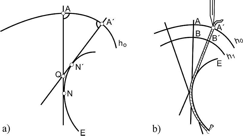
Figure 2 a) Construction of the family of curves of common evolute curve. b) Formation of the curves’ family. 

Let NA and N'A' be two norms to the curve h_o, which intersects on Q. If A and A' are two points, which are very close to each other over h_o, then the curve described by NQ+QN' can be approximated by the arc ∪NN', and from Fig. 2a) we have

(1)

Since A and A' are very close together, then A'Q = AQ, and, as a consequence, ∪NN'=(AN-A'N'), resulting in

AN=∪NN'+A'N' (2)

Equation (2) allows us to think of a thread rolled to the evolute curve passing by N', following the segment N'A', so that its end point is on A'. Since ∪NN'=(AN-A'N'), the point A' can be moved to the point A, describing the curve h_o, see Fig. 2b. The same can be done for points B' and B by changing the length of the thread, but, in this case, the described curve will be h_i, which has the same evolute as h_o. By making different increments of the length of the thread, a family of curves having the same evolute can be generated.

2.2. Family of curves of common parallel

A parallel curve has the property to maintain a certain distance, measured over the norm of the curve in each point, from another curve. From this definition is evident that the proposed family of curves of common evolute is at the same time a family of curves of common parallel. To picture this, let us suppose a support curve, f(t), and a parallel curve, g(t), that is generated at a distance r from f(t), as seen in Fig. 3.

Figure 3 Parallel curve g(t). 

The condition to generate parallel curves to a given curve is that it must be regular. If the initial curve, represented in its parametric form, f(t) = (x(t), y(t)), then the parallel curve to it is given by

(3)

where

n(t)=1‖f'(t)‖(-y'(t),x'(t))

is the curve’s normal vector, r is the distance between the curves f(t) and g(t), and f'(t) = (x'(t), y'(t)).

The derivative of the vector g(t), is given by

g'(t)=(1-rTf(t))f'(t) (4)

where the curvature of the curve f(t) is of the form,

Tf(t)=x'(t)y″(t)-x″(t)y'(t)‖f'(t)‖3

From Eq. (4), we can say that if f(t) is a regular curve, as long as r^-1 does not belong to the range Tf(t), g(t) will also be a regular curve. The relationship between the curvatures tures of f(t) and g(t), and Tf(t) and Tg(t), can be shown by derivating such equation,

(5)

then

Tg(t)=‖g'(t)g″(t)‖‖g'(t)‖3=(1-rTf(t))2‖f'(t)f″(t)‖)|1-rTf(t)|3‖f'(t)‖3 (6)

which represents the curvature of the parallel curve.

If f(t) is a closed curve, g(t) will also be a closed curve. The regularity property of f(t) can be lost in g(t), depending of the existence of the roots of the equation (1-rTf(t))f'=0, in the g(t) domain ¹².

2.3. Family of curves of common parallel with common evolute generated from an ellipse

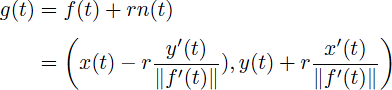
If the parallel curves use an ellipse as a support curve, then by setting the major semi-axis of the ellipse as a and the minor semi-axis as b, we obtain

f(t)=(x(t),y(t))=(acos⁡(t),b sen(t)), (7)

with a travel path of (0,2π), resulting in x'(t) = -a sen(t) and y'(t) = b cos(t). Taking into account Eq. (3) and the curvature Tf(t), and by substituting the values of the parametric equations and their derivatives into them, the expression for the family of parallel curves (for each value of r) is of the form

g(t)=acos⁡(t)-rbcos⁡(t)(a2 sen2(t)+b2cos2⁡(t))12b sen(t)-rasen(t)(a2 sen2(t)+b2cos2⁡(t))12, (8)

where

Tf(t)=ab(a2 sen2(t)+b2cos2⁡(t))32.

The curvature for the regular curve g(t) is given by,

Tg(t)=±ab(a2sen2(t)+b2cos2⁡(t))32-rab, (9)

where the plus sign (+) corresponds to the case in which r < b²/a and as a result 1-rTf(t)>0. The minus sign (-) corresponds to the case where < a²/b , which is a minimum absolute, and, therefore, 1-rTf(t)<0. By analyzing the support curve, we have that the absolute extrema of this function in the interval (0,2π) are reached at:

Tf0= ab2,   the maximum absolute, and (10)

Tf(π/2) =Tf(3π/2)=ba2,   the minimum absolute. (11)

Then, the limits of r for the curve to be regular are: a²/b ≤ r ≤ b²/a.

It is clear, that every parallel curve to f(t) with r < 0 is regular, since Tf(t)>0 and, thus, 1-rTf(t)>0. Figure 4a) shows that for every r < b²/a the obtained curves are regular and have the same geometry of the support curve.

Figure 4 Parallel curve of the elliptical curve for: a) r < b²/a y b) r < a²/b. 

Also, the parallel curves for the same support curve but for r < a²/b , are regular curves too, see Fig. 4b).

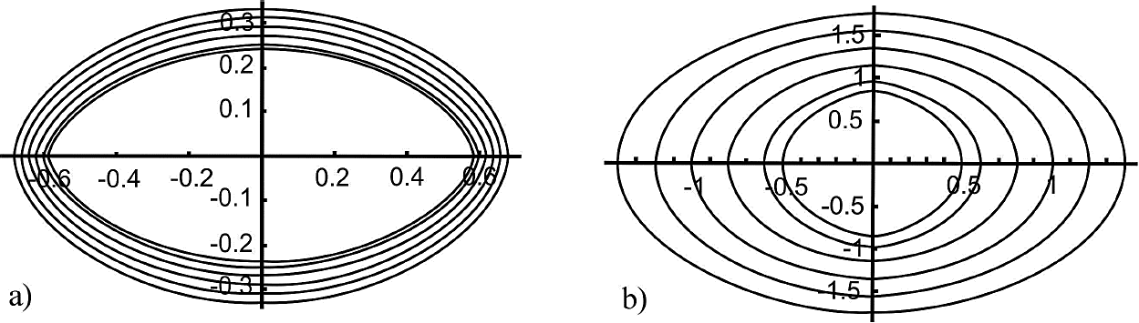
It can be seen from Fig. 4 that, as we approach to the center of the ellipse, its parallel curves start suffering changes. These changes are more pronounced when the parallel curves are in the range of b²/a < r < a²/b, where they stop being regular. At this point, the parallel curves start to intersect each other and to change their direction. The parallel curve cuts at the x-axis origin when r = b, see Fig. 5b), and when r = a the curve cuts at the y-axis origin, as shown in Fig. 5c). As r continue growing the curve becomes regular until r = a²/b.

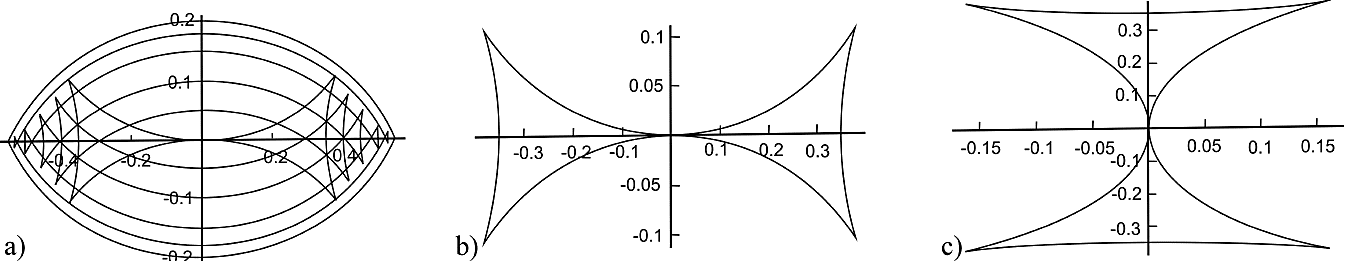
Figure 5 a) Auto-intersections of the parallel curves at the x-axis. b) Parallel curve cutting at the origin on the x-axis. c) Parallel curve cutting at the origin on the y-axis. 

The cuts at x and y can be seen from Eq. (8). Centering our attention onto the cut at the x-axis, we have

y=b sen(t)-rasen(t)(a2sen2(t)+b2cos2⁡(t))1/2=0. (12)

From Eq. (12) the intersections of the curves with the x-axis are seen. This equation has two roots (t = 0 y t = π), but if

b-ra(a2sen2(t)+b2cos2⁡(t))1/2=0.

then there are two more roots that can be obtained. If r < 0, these roots do not exist, and the outwards ellipse parallel curves cut the x-axis only at t = 0 and t = π, then by taking into account only r > 0, we have

sen2(t)=r2a2-b4b2a2-b4=0. (13)

These t values exist and are different from 0 and π, if and only if,

0<r2a2-b4b2a2-b4<1,

so

t= arcsenr2a2-b4b2a2-b41/2,

i.e., that in b²/a < r < b an intersection of the g(t) curve with the x-axis exists, and we are at the origin when r = b, see Fig. 5.

In analogy, it can be seen that g(t) also has two intersections with the y-axis, at t = π/2 and at t = 3π/2, which comes from Eq. (8) when x = 0. As a result, the cut on the y-axis is:

x=acos⁡(t)-rbcos⁡(t)(a2sen2(t)+b2cos2⁡(t))1/2 (14)

where

a-rb(a2sen2(t)+b2cos2⁡(t))1/2=0. (15)

There are no intersection for the case in which r < 0 and therefore

cos2(t)=a4-r2b2a4-b2a2.

The latter values can only exist, if and only if,

0=a4-r2b2a4-a2b2.

2.4. Non-conventional zone plate of common parallel

In order to design a non-conventional zone plate of common parallel, we chose an ellipse as a support curve. The family of ellipses has a separation in between the curves of n,

f(t)=(a+n-1)cos⁡(t),(b+n-1)sen(t), (16)

from this equation we can see that

xn=a+n-1cos⁡t=ancos⁡t andyn= (b+n-1)sen(t)=bncos⁡(t), (17)

where n can take the values of 1, 2, 3, 4,…, etc., which means that, for each n, we will have a ring. The zone plate presented in this work has 20 rings, i.e., n = 20, see Fig. 6b). And, the family of parallel curves is

g(t)=ancos⁡(t)-rbncos⁡(t)(an2sen(t)2+bn2cos⁡(t)2)1/2bn sen(t)-ransen(t)(an2sen(t)2+bn2cos⁡(t)2)1/2 (18)

and the curvature of the n-th curve is given by

Kgn(t)=±anbn(an2sen(t)2+bn2cos⁡(t)2)3/2-ranbn. (19)

Figure 6 a) Experimental setup. b) Non-conventional zone plate of common parallel. 

3. Experimental setup and results

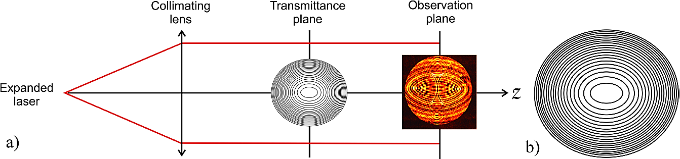
In order to obtain the transmittance of Fig. 6b), computational software was used. The resultant graphic was printed on a white paper sheet, then it was photographed and reduced at (1:30) onto a high resolution plate (HRP). The size of the resultant transmittance was < 5 mm².

The characterization of the non-conventional zone plate was carried out by using the experimental setup shown in Fig. 6a). The obtained results are shown in Fig. 7.

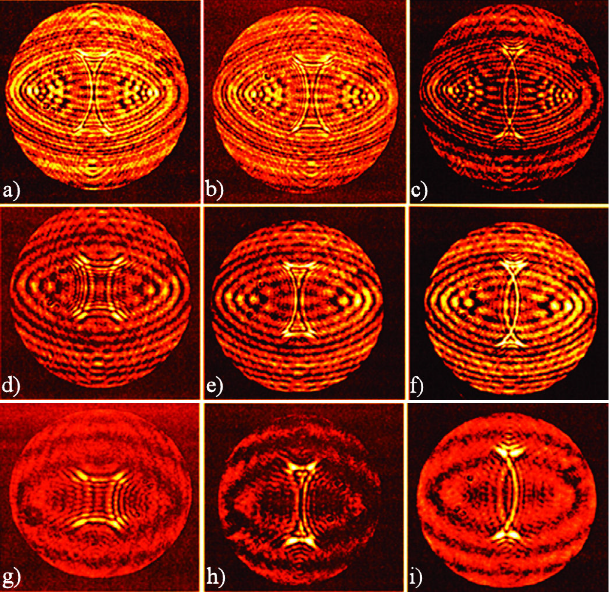
Figure 7 Evolution of the propagated field using the non-conventional zone plate of common parallel at the following distance from the transmittance: a) 3.1 cm, b) 3.4 cm, c) 3.7 cm, d) 7.4 cm, e) 7.8 cm, f) 8.1cm, g) 10.9 cm, h) 11.1 cm, i) 11.6 cm. 

The results shown in Fig. 7 are in total agreement with the theory. By observing images b), e), and h) taken in different propagation planes, we can see the existence of auto-images. The same thing happens in the case of images c), f), and i).

4. Discussion

The focalization of the constructed zone plate can be explained based on the geometrical and mathematical descrip- tion of Sec. 1 and 2, which gives as a result that the generated family of curves has a common evolute as well as a same common parallel.

Since the non-conventional zone plate is a transmittance plate, which is illuminated by a coherent plane wave, and by taking the Huygens principle and the Fresnel postulate into account, then the points in which the secondary waves interfere in a constructive way can be considered.

Having the support curve, f_o , we follow the propagation of a ray that travels perpendicular to the curve. The same procedure is done for different rays and an instant of time later we can see how the wavefront has evolved, points A, B, and C of Fig. 8. By definition these points fall on the parallel curve g(t), i.e., the parallel curve g(t) is a wavefront.

Figure 8 Analysis of the evolution of the family of curves, f_o and f₁, of common parallel g(t). 

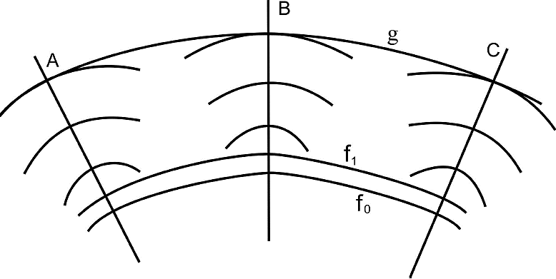
Let us analyze the emission of the second curve that constitutes the family of curves f_o and f₁. Due to the fact that both of them have the same evolute and share the same family of perpendicular lines for each propagation plane, the wavefront coming from f₁ has a constant phase difference with respect to the one coming from f_o. If the phase difference is such that the wavefronts interfere in a constructive way, then the geometrical focalization point will correspond to a parallel curve, such that

where Δr = mλ.

On the arbitrary points A, B, and C we will have a group of parallel curves with a certain geometry of focalization; we just need to make a displacement of r + Δr to move to a different curve. Since r is a continuous parameter, the generation of these curves is in the entire propagation plane. Each of these curves has a constant phase, which is repeated by a modulus of 2π. Due to the latter, the generated family of curves replicates itself as shown in Fig. 7. This self-image or replica of the geometries is due to the periodicity of the constructive interference regions. The total field for a certain detection plane is formed by the superposition of the envelope curve and the corresponding parallel curve for such a displacement. If the propagation plane changes, a new parallel curve will be obtained, as it has been seen.

The perpendicular rays associated to the parallel curves, which are generated by the constructive interference of the emission of the family of curves that constitutes the zone plate along the propagation axis, have the same envelope, i.e., a caustic. The latter gives us an insight that we are obtaining the evolution of the focalization region organizing itself in the surroundings of the caustic.

5. Conclusions

The focalization properties of the constructed non-conventional zone plate, evolving as parallel curves along the propagation axis, are explained by using the Huygens-Fresnel principle. The Fresnel diffraction patterns can be seen as the redistribution of energy in a successive parallel curves evolving along the propagation axis. The focalization regions are seen as points of constructive interference and the evolute as the normal envelope of the rays.

This treatment can be applied to some other type of support curves, not only elliptical, which means that this method can control the geometry of the focalization region by changing the support curve used to generate the focalization diffraction element. As a result, the diffraction element can be customized in order to obtain a specific focalization field.