


 nova página do texto(beta)
 Inglês (pdf)
 Artigo em XML
 Referências do artigo
 Enviar este artigo por email
 Citado por SciELO
  Similares em
SciELO
Similares em
SciELO 
 Permalink
Introduction
Electrical resistivity investigation techniques are extensively used for several applications, among others, water exploration to search suitable groundwater sources or groundwater pollution, engineering prospection to locate sub-surface faults, fissures and cavities, permafrost, etc, and archaeological mapping to define the extension of buried formations or ancient buildings (Reynolds, 2011). They are used in those fields to obtain detailed information readily and economically about the location, depth, and resistivity of subsurface formations. Those electrical resistivity techniques applied on the surface have proved to successfuly delineate the subsurface geology and structures (Olasehinde, et al., 2013).
The traditional Vertical Electrical Sounding (VES) with Schlumberger configuration is an effective electrical resistivity surveying technique for groundwater exploration (Edwards, 1977 and Zohdy et al., 1984).
The one-dimensional (1D) quantitative interpretation of the VES measurements allows the real resistivities and thicknesses to be determined under every studied VES point (Zohdy and Bisdorf, 1989). The two-dimensional (2D) qualitative VES interpretations are mainly oriented towards establishing the geoelectrical section and analyzing the resistivity variations along a given profile laterally and vertically, where the 1D quantitative VES results are used for such a 2D interpretation. Establishing a 2D interpretation analysis is not an easy task, because every VES point is solely 1D interpreted without considering the effect of other surrounding VES. In those conditions, the 2D interpretations along a given VES profile strongly depend on the experience of the geo-scientist and his geological knowledge of the study region. Such a weakness prevents giving an accurate and integrated subsurface geoelectrical picture, particularly in geologically complex areas, and in the area between the interpreted VES along the studied profile.
The Pichgin and Habibulleav method (1985) enhanced by Asfahani and Radwan (2007) is one of the elaborated mathematical techniques for interpreting VES measurements distributed along a given profile in terms of a two-dimensional model (2D). It has been successfully applied in Syria for solving different structural subsurface problems related to groundwater (Asfahani and Radwan, 2007), and in geo-exploration mining such as phosphate, uranium, sulfur, and bitumen (Asfahani, 2010; Asfahani, 2011). This 2D method has been recently applied by Al-Fares and Asfahani (2018) for solving the Abou Barra leakage dam problem in Northern Syria. It was also applied in the Arbil region for environmental and groundwater contaminations studies (Gardi and Asfahani, 2018). This 2D technique is oriented towards determining in detail the structural subsurface along a given VES profile.
A new procedure for the interpretation of VES data with the use of a 1.5D simultaneous inversion method was proposed by Gyulai and Ormos in 1999. The basic idea of their method showed that the horizontal changes in the layer thicknesses and the resistivities of the 2D geological structure can be described by (expanding in series) functions of spatial coordinates. The coefficients of the basis functions are determined from the VES data by a simultaneous inversion method using a least-squares technique.
A quick 2D geoelectric inversion method using series expansion was also proposed by Gyulai et al., 2010. They indicated that horizontal changes in the layer-thicknesses and resistivities of the geological structure are discretized in the form of series expansion. The linearized iterative least-squares (LSQ) inversion of data provided by surface geoelectric measurements determines the unknown expansion coefficients. The discretization of the 2D model using series expansion gives the possibility to reduce the number of model parameters. The resulting inverse problem becomes consequently over-determined and can be solved without the application of additional regularization.
A combined geoelectric weighted inversion was proposed by Gyulai et al., 2014 for interpreting VES data for environmental exploration purposes. The 2D combined geoelectric inversion (CGI) method performs more accurate parameter estimation than conventional 1D single inversion methods by efficiently decreasing the number of unknowns of the inverse problem (single means that data sets of individual vertical electric sounding stations are inverted separately).
Gyulai et al., 2016 used 2.5D CGWI combined geoelectric weighted inversion of VES measurements for characterizing geoelectrically the thermal water aquifers. According to their technique, which uses the joint 2D forward modeling of dip and strike direction data, the 3D structures can be determined.
A new geoelectrical combined sounding-profiling configuration was recently adapted and proposed for increasing the resolution of 1D VES quantitative interpretations (Asfahani, 2018). The electrode C in this new proposed three-electrode array is not fixed at the infinity but is slightly modified and movable, where OA=OB=OC=AB/2 as shown and presented in Figure 1. It allows to gain a maximum of geoelectrical information when ρAB gradient transformation and ρAC/ρBC are integrally interpreted, to get an accurate subsurface resistivity picture along a given profile.
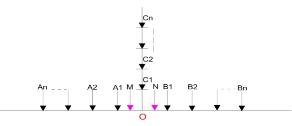
Figure 1 Schema of the combined sounding- profiling configuration (two three electrode configurations AMN and MNB). A, B and C: current electrodes, M and N: potential electrodes, O: configuration center (Asfahani, 2018).
The geo-electric surveys have been carried out in the Khanasser valley in Northern Syria for hydro-geological purposes to solve different posed problems in the study region. The VES technique applied in this survey is oriented to provide information concerning the thickness of subsurface layers, geological structures, contributing groundwater occurrence, and to follow the lateral and vertical variations of subsurface layers. Those VES measurements have been carried out during an international cooperation program, which has been established between three scientific organizations; ICARDA, AECS, and Bonne university (Schweers et al., 2002). The objectives of this program have been designed to address the typical problems characterizing the marginal dry-land environments. The poverty, the relatively easy accessibility, and the diversity and dynamics of the natural resources and livelihoods made Khanasser valley region a prime candidate.
The present paper discusses an application of the geoelectrical survey using Schlumberger VES technique, oriented towards clarifying and identifying the subsurface resistivity variations in terms of a 2D semi-quantitative interpretation along a given profile.
A fractal modeling technique adapting the concentration- number (C-N) model is proposed herein as a new approach to interpreting the geoelectrical VES measurements carried out along a given profile. It is worth mentioning that the same fractal modeling technique (C-N) was recently applied for characterizing the basalt environments in Southern Syria, where different geological scenarios have been established and proposed to explain the basalt distributions along different profiles in the study region (Asfahani and Al-Fares, 2021).
Different geoelectrical profiles (LP1, LP2, LP3, and TP5) are selected from the study Khanasser valley region (Fig. 2 and Fig.3), and re-interpreted by using this new fractal approach.


The fractal and multifractal models developed by Mandelbrot (1983) are widely used in different branches of geosciences. Those models are used for example in geophysical exploration for the separation of geophysical anomalies from background. Fractal dimensions of variations in geophysical resistivity data can therefore provide useful information and applicable criteria to identify and categorize different lithological zones within the studied profiles. The log-log plots are suitable to distinguish between different resistivity populations, and make a kind of classification in the geoelectrical data. In fact, the threshold values determined can be identified and delineated as break points in those log-log plots. A break point located and determined in the log-log plot reflects a lithological change and the passage from a lithology to a different one. The determination of those points makes the fractal C-N model more precise, being very sensitive to the lithological boundary location.
The concentration-number (C-N) fractal model is applied and newly introduced in this paper to distinguish between different resistivity populations, and give a range of resistivity values for each of them. Such a new application makes the unclear apparent resistivity values obtained as a function of depth (AB/2) to a clearer litho-resistivity populations, easily explained and documented along a given profile.
In this way, a semi-quantitative technique is proposed herein for interpreting the resistivity variations with depth using the VES technique along a given profile.
The main objectives of this paper are therefore constructed to be as follows:
1) Carrying out VES measurements distributed along given profiles with Schlumberger array.
2) Proposing the fractal modeling technique as a new approach to interpret VES measurements carried out along a given profile.
3) Interpreting the measured VES data points by using the new proposed approach and the 2D concentration-number (C-N) fractal model with the log-log plots, to get a kind of litho-resistivity pseudo section for the VES measurements distributed along a given profile.
4) Comparing the VES results obtained by the fractal modeling with other traditional geoelectrical interpretations.
Hydrogeology of the Khanasser Valley
Khanasser Valley is located approximately 70 km southeast of Aleppo City, and lies between two hill ranges; the Jabal Shbeith eastwards and the Jabal Al Hoss westwards. The southern part drains towards the Adami depression in the south, while the northern part of the valley drains towards the Jaboul Salt Lake (Figs. 2 and 3).
Three aquifers are used in the Khanasser Valley for groundwater extraction. The deepest is of upper Cretaceous age at 400 m below ground level. Above the Maestrichtian, the Paleocene-Lower Eocene limestone aquifer of low productivity is located (ACSAD, 1984), where the average hydraulic conductivity (k) as referred from the pumping test is 0.0054 m/day (Schweers et al., 2002). Lengiprovodkhoz (1987) had previously registered a hydraulic conductivity ranging between 0.008 m/day and 0.5 m/day for the Paleogene formation. The paleogene strata in the central part of Khanasser valley are not very thick; about 50 m of lower Eocene and Paleocene overlay the Maastrichtian. Quaternary water-bearing formations, the most transmissive in the region situated near the surface, are covered by some of 10 m of alluvial and proluvial soil. This aquifer receives direct recharge from rainwater as well as infiltrating runoff and subsurface flow from the slopes of Jabal Al Hoss and Jabal Shbeith. Electrical conductivities of groundwater in this aquifer vary between 2.5 and 26 dS/m, (Schweers et al., 2002).
Figure 4 shows a geological section of NW-SE orientation from Jabal. Al Hoss to Jabal. Shbeith passing through Khanasser Valley, in which the different geological formations with their stratigraphic units are presented.
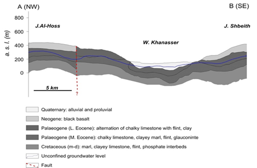
Figure 4 Geological section of NW-SE orientation from Jabal.Al Hoss to Jabal.Shbeith passing by Khanasser Valley.
The rapid development of mechanical irrigation wells during the last two decades has led to a substantial increase in groundwater withdrawal from the upper, unconfined aquifer system. The groundwater monitoring and analysis indicate that the valley may be affected by salt water intrusion from the Jaboul Salt Lake, where variable changes in water level and quality are observed since 1998 (Hoogeveen and Zobisch, 1999; Asfahani and Abo Zakhem, 2013). Rainfall is comprised between 200 and 250 mm/year and is not predictable, while the natural resources are quite poor and prone to degradation.
Vertical Electrical Soundings (VES)
VES technique requires to impose an electrical current on the study area by a pair of A and B electrodes at varying spacing expanding symmetrically from a central point, and to measure the surface expression of the resulting potential field with an additional pair of M and N electrodes at appropriate spacings.
The apparent resistivity (ρa) is expressed by the following equation:
Where I is the current introduced into the earth by A and B electrodes, and ΔV is the potential measured between the potential electrodes M and N, as shown in Fig. 5.

The electrical (VES) sounding gives an estimate of the variation of the electrical resistivity with the depth below a given point on the earth surface. Fig. 6 shows the field resistivity curve measured at point V10-4, which plotting the apparent resistivity values (ρa), obtained by increasing the electrode spacing (AB/2) about a fixed VES point (ρa= f (AB/2)).

The field apparent resistivity curve is interpreted using a curve matching technique of master curves (Orellana and Mooney, 1966), where an initial approximate model of thicknesses and resistivities of corresponding layers is obtained. This approximate model is thereafter accurately interpreted with an inverse technique program until reaching acceptable goodness of fit between the field resistivity curve and the theoretical regenerated curve (Zohdy, 1989, Zohdy and Bisdorf, 1989).
Field survey
An Indian equipment (ACR-1) has been used to survey ninety-six VES points in the study region, distributed on a grid including three longitudinal profiles labeled as LP1, LP2, and LP3, and nine transverse profiles oriented approximately NW-SE (Fig. 3) and labeled as (TP1, TP2, TP9). The resistance (ΔV/I) is directly measured by the ACR-1, and the apparent resistivity (ρa) is consequently estimated according to equation [1] (Dobrin, 1976). The distance between profiles is approximately 1 km, where a VES point is generally measured every kilometer along each profile (especially in the valley itself). This distance observation interval is sometimes changed according to the topographic conditions. The geo-electrical lines for all the VES executed in the study area have been chosen to be parallel to the direction of Khanasser valley axis of N301E. Schlumberger array was applied to carry out those ninety-six VES measurements, for which a maximum current electrode spacing (AB/2 = 500 m) of 1000 m was used.
Fractal Theory
Mandelbrot (1983) has already proposed the fractal geometry with its different models, as a nonlinear mathematical science, to be extensively practiced in many branches of earth sciences. Different applications of 2D and 3D geophysical data have been carried out by using several fractal-multifractal models, which have been recently proposed, such as concentration-number (C-N) (Hassanpour and Afzal, 2013), concentration-distance (C-D) (Li et al., 2003), and concentration-volume (C-V) (Afzal et al., 2011).The application of the fractal models requires the use of log-log plots, in which the straight line segments fitted to the log-log graph have some break threshold points (Zuo, 2011; Wang et al., 2011; Mohammadi et al., 2013). Every straight line segment determined on the log-log plots reflects a specific geophysical population, that we have to evaluate its variation range.
The (C-N) multifractal model is proposed in this paper as a new application approach for interpreting the VES measurements distributed along a given profile, and explaining its resistivity variations with depth through differentiating between different resistivity ranges. The concentration-number (C-N) fractal model is expressed by the following equation:
Where ρ denotes the treated geoelectrical parameter values. The geoelectrical parameter used in this paper is the apparent resistivity (Ω.m). N(≥ρ) denotes the cumulative number of the apparent resistivity data (Acρ), with the resistivity parameter values greater than or equal to ρ, F is a constant and D is the scaling exponent or fractal dimension of the distribution of electrical resistivity parameter values.
Results and discussion
The ninety-six (VES) measurements carried out in the Khanasser Valley have been firstly 1D interpreted by using the master curves, where an initial approximate model with resistivities and thickness of corresponding layers are reached (Asfahani, 2007). The reached approximate model is secondly interpreted by an inversion resistivity program for getting correctly the final optimum theoretical curve, that fits as best as possible with the measured apparent resistivity data. The geological layers in the field in such a 1D quantitative interpretation are assumed to be horizontal (Asfahani, 2007). Fig.6 shows an example of field VES curve obtained at the point V10-4 and its interpretative model solution. The ninety six (VES) measured points were distributed on twelve profiles as shown in Fig. 3 and interpreted with the assumption of 1D structure (Asfahani, 2007). Three of those profiles are longitudinal, labeled LP1, LP2 and LP3 and carried out in the Khanasser valley itself, while the other nine are transverse and labeled TP1, TP2, and TP9. The thickness and resistivity parameters of the Quaternary and Paleogene deposits are quantitatively evaluated through interpreting those ninety six measured (VES) points (Asfahani, 2007). The Quaternary deposits thickness varies between a minimum of 4.5m and 99.4m with an average of 38.5 m. Its resistivity varies between 4.1 and 43 Ω.m with an average of 15.3 Ω.m. The Paleogene thickness varies between a minimum of 54m and a maximum of 283m, with an average of 162.4 m. Its resistivity varies between 1.7 and 16 Ω.m with an average of 5.1 Ω.m (Asfahani, 2007).
The Pichgin and Habibullaev (1985) method has been already applied for interpreting the VES soundings distributed along the mentioned longitudinal and transverse profiles in term of 2D modeling (Asfahani and Radwan, 2007). This 2D interpretation modelings have already allowed to get detailed subsurface images about the studied profiles. Fig. 7 shows an example on using this 2D technique for interpreting LP2 profile. According to this technique, the subsurface tectonic fractured zones, and the geological structural features for all the AB/2 spacings have been defined along LP2 profile.

The results of this interpretative method as previously explained (Asfahani, 2007; Asfahani, 2010) are presented by the points of nonhomogeneity (+), which mainly show the locations of fractured zones as shown under the V4-3 and V5-4 soundings, and under the V8-2 and V10-2 soundings. The distribution of these points in regular form of bedding planes as shown between the V8-2 and V6-2 soundings reflects the geological structure of the study area. It is evident that the Maastrichtian formation is remarkably uplifted. The effect of the Quaternary paleo-sabkhas discussed previously is also shown under the V10-2 in the north. Other similar tectonic subsurface features have also been traced through the analysis of the other two measured profiles LP1 and LP3 (Asfahani, 2007).
The three longitudinal profiles LP1, LP2, and LP3 and the transverse TP5 profile are studied, analyzed, and re-interpreted in this paper, by applying the proposed multifractal (C-N) modeling technique. The application of the multifractal modeling technique is considered as a new approach for getting a semi-quantitative interpretation for the VES soundings distributed along a given profile. It allows having a preliminary idea about the number of apparent resistivity populations, present along the studied profile.
The LP1 profile of length of 23.77 Km includes eleven VES measured points, for which the resistivity variations as a function of AB/2 varying from 3 to 500 m are analyzed and interpreted by the use of fractal concentration-number (C-N) model. Based on the C-N log-log plot presented in (Fig.8) for LP1 profile, the 176 data points of apparent resistivity ρa for all the AB/2 (from 3 to 500 m) show three threshold break points C1, C2, and C3 at 1, 1.16, and 1.36 respectively. The log (ρa) values indicate an apparent resistivity of 10, 14 and 23Ω.m respectively.

The log-log plots of Acρ as a function of the apparent resistivity values show the scattered data points, which can be fitted by several straight lines (segments) with different slopes based on a least square regression. The selection of the break points as threshold values is an objective decision since apparent resistivity populations are addressed by different line segments in the C-N log-log plots. The intensity of various populations is depicted by each slope of the line segment in the C-N log-log plots.
Those three break points correspond to four apparent resistivity ranges as follows: the first range is less than 10 Ω.m, the second range is between 10 and 14 Ω.m, the third range is between 14 and 23 Ω.m, and the fourth range is bigger than 23 Ω.m. The use of those resistivity ranges allows the establishment of the apparent resistivity cross section along LP1 profile as shown in Fig. 9B. The distinction between those four resistivity populations is clear, where every resistivity population is due to a distinct and specific lithology. The boundaries between those resistivity ranges also emphasize indirectly the lithologic type distribution along the studied profile. Geological interpretation about the lithology and the resistivity population could be easily done along the studied LP1 profile. By such a manner, a semi quantitative 2D interpretation could be achieved. The traditional iso-apparent resistivity map is established as a function of AB/2 along the LP1 profile as shown in Fig.9A. The distance in kilometer along LP1 profile is represented linearly, while the depth of AB/2 in meter is represented with a negative sign in a logarithmic scale to get an acceptable concordance between the two axes (distance and depth). The scale of AB/2 being logarithmic, the corresponding AB/2 of -3, -4.3, -5.2, -6.15, -7.25, -8.1, -9.1, -9.9, -10.5, -11.4, -12.3, -13.4, -14.2, -15.3, -16.1, and -16.7 are used instead of AB/2 of 3, 5,7, 10, 15, 20, 30, 40, 50, 70, 100, 150, 200, 300, 400, and 500 m, respectively.
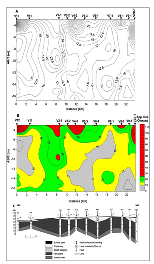
Figure 9 A: Traditional iso-apparent resistivity cross section along LP1 profile. B: Concentration-number fractal model along LP1 profile. C: Traditional 1D quantitative geoelectrical model along LP1(Asfahani, 2007).
The iso-apparent resistivity map shown in Fig.9A is difficult to be qualitatively interpreted, compared with that obtained by applying the multi-fractal approach (Fig.9B). It is worth mentioning that an acceptable coincidence is obtained between the multi-fractal established apparent resistivity cross-section along LP1 profile (Fig.9B) and the traditional 1D quantitative interpretation along this LP1 profile, as shown in the figure 9C (Asfahani, 2007). The VES sounding at V6-1 point for example shows four resistivity populations from up to down. The first one is related to the resistivity range of bigger than 23 Ω.m, and reflects the superficial layer. The second range of between 10 and 14 Ω.m, and the third range of between 14 and 23 Ω.m represent the Quaternary deposit, separated in this V6-1 point into two distinguished layers. The first resistivity range of less than 10 Ω.m indicates to the Paleogene presence. This V6-1 point was 1D quantitatively interpreted adapting a model of 5 layers (Asfahani, 2007). The resistivity of the first superficial layer is 26.8 Ω.m and its thickness is 3.7m. The second layer has a resistivity of 8.5 Ω.m and a thickness of 34.7 m; The third layer has a resistivity of 25.8 Ω.m and a thickness of 49.4 m, and both of them are of Quaternary deposit with different resistivities. The fourth layer related to the Paleogene has a resistivity of 5.7 Ω.m and a thickness of 226 m. The fifth layer is related to the Maastrichtian and has a resistivity of 51 Ω.m. This quantitative described model for V6-1 has been completely indicated, shown, and confirmed by the fractal concentration-number model, where a good coincidence is obtained between the two different interpretative approaches.
The Paleogene is shown near the surface at V7-1 directly after the superficial layer of a resistivity of 16 Ω.m and thickness of 6 m.
The application of the proposed fractal (C-N) approach on the 192 apparent resistivity data points related to LP2 profile shows three threshold break points of C1, C2, and C3 at 0.78, 1.16, and 1.39 respectively as presented in (Fig.10). The log (ρa) values indicate an apparent resistivity of 6, 14 and 24 Ω.m, respectively. Those three break points correspond to four apparent resistivity ranges as follows; the first range is less than 6 Ω.m, the second range is between 6 and 14 Ω.m, the third range is between 14 and 24 Ω.m, and the fourth range is bigger than 24 Ω.m. The established apparent resistivity cross-section along LP2 profile is illustrated in Fig.11B.

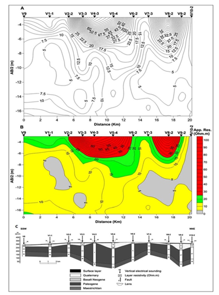
Figure 11 A. Traditional iso-apparent resistivity cross section along LP2 profile. B: Concentration-number fractal model along LP2 profile. C: Traditional quantitative geoelectrical model along LP2 (Asfahani, 2007).
The iso-apparent resistivity map established as a function of AB/2 along LP2 shown in Fig. 11A is also difficult to be qualitatively interpreted in comparing with that obtained by applying the proposed multi fractal approach (Fig.11B). An acceptable coincidence between the multi fractal established apparent resistivity cross-section along LP2 profile (Fig.11B) and the traditional 1D quantitative interpretation along this LP2 profile is also obtained, as shown in Fig. 11C (Asfahani, 2007).
The application of fractal approach (C-N) on the 192 apparent resistivity data points related to LP3 profile indicates four threshold break points of C1, C2, C3 and C4 at 0.75, 0.98, 1.24 and 1.43 respectively as shown in Fig.12. The log (ρa) values indicate an apparent resistivity of 5.6, 9.5, 17.4 and 30 Ω.m respectively. Those four break points correspond to five apparent resistivity ranges as follows; the first range is less than 5.6 Ω.m, the second range is between 5.6 and 9.5 Ω.m, the third range is between 9.5 and 17.4 Ω.m, the fourth range is between 17.4 and 30 Ω.m. The fifth range is bigger than 30 Ω.m. The established apparent resistivity cross-section along LP3 profile is shown in Fig. 13B. The same remarks as documented on LP1 and LP2 profiles could be shown with LP3 profile. The iso-apparent resistivity map established as a function of AB/2 along LP3 shown in Fig. 13A is also difficult to be qualitatively interpreted when compared with that obtained by applying multi fractal approach.

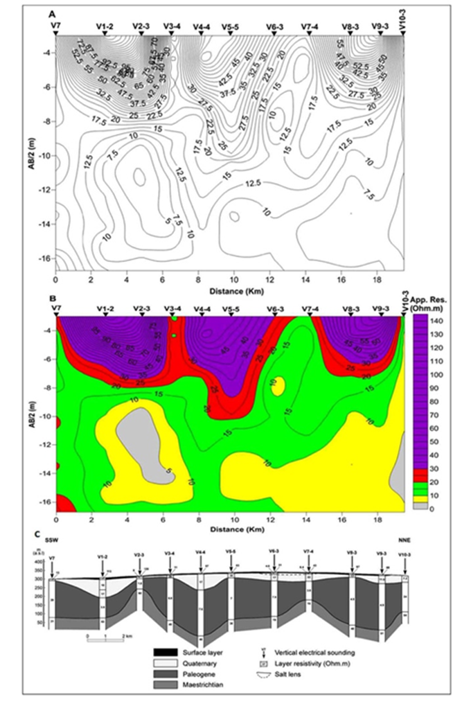
Figure 13 A. Traditional iso-apparent resistivity cross-section along the LP3 profile. B: Concentration-number fractal model along with LP3 profile. C: Traditional quantitative geoelectrical model along LP3 (Asfahani, 2007).
The application of fractal (C-N) approach on the 144 apparent resistivity data points related to the transverse TP5 profile shows four threshold break points C1, C2, C3 and C4 at 1, 1.19, 1.44 and 1.70 respectively as presented in Fig.14. The log (ρa) values indicate an apparent resistivity of 10, 15, 27.5 and 50 Ω.m respectively. Those four break points correspond to five apparent resistivity ranges as follows: the first range is less than 10 Ω.m, the second range is between 10 and 15 Ω.m, the third range is between 15 and 27.5 Ω.m, the fourth range is between 27.5 and 50 Ω.m. The fifth range is bigger than 50 Ω.m. The established apparent resistivity cross-section along TP5 profile is illustrated in Fig.15A.
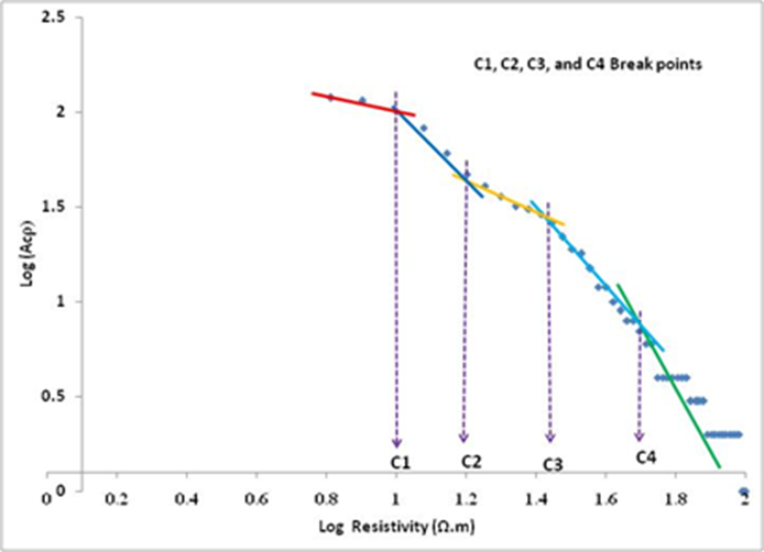
Figure 14 Fractal C-N log-log plot for the measured apparent resistivity data along the TP5 profile.
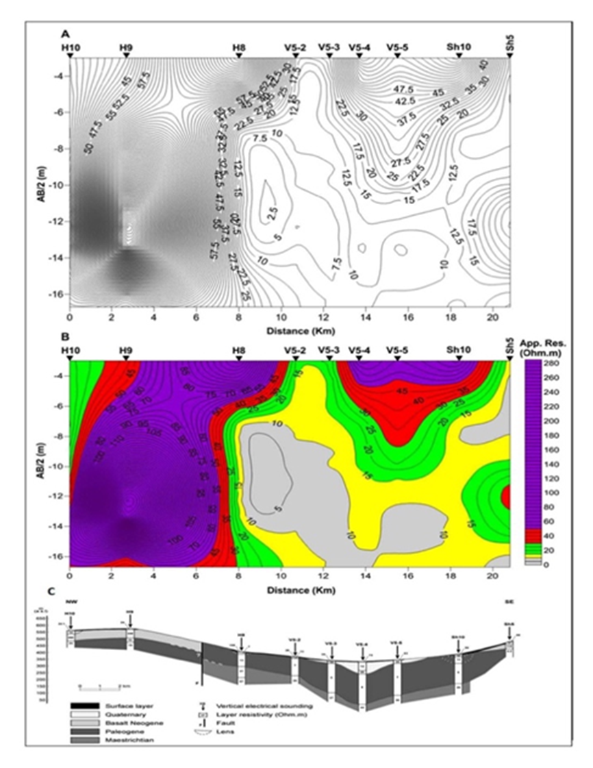
Figure 15 A. Traditional iso-apparent resistivity cross section along TP5 profile. B: Concentration-number fractal model along TP5 profile. C: Traditional quantitative geoelectrical model along TP5 (Asfahani, 2007).
The above-treated examples and the different comparisons shown between the established multifractal cross-sections and the traditional 1D quantitative interpretative models along the studied profiles LP1, LP2, LP3, and TP5 confirm the feasibility of the new proposed fractal approach.
Validation of the C-N technique
The fractal C-N modeling approach is a nonlinear tool that deals with field apparent resistivity measurements to separate different apparent resistivity ranges, that differ from one profile to another. This approach is newly introduced in this research to interpret in terms of 2D modeling the VES measurements distributed along a given profile.
Traditionally, the field apparent resistivity measurements of each VES point have been treated and interpreted separately using different known inversion procedures. The inversion allows consequently to obtain a one-dimensional (1D) interpretation model including the real thicknesses and resistivities of the layers under the study VES point. On the other hand, when the fractal C-N modeling procedure is applied, all the apparent resistivity measurements distributed under a given profile for all AB/2 spacings are treated together at the same time by the use of log-log plots, as demonstrated above during interpreting the four profiles (LP1, LP2, LP3, and TP5). The use of the fractal C-N model with the log-log plots permits to determine the break points and the different line segments with their related apparent resistivity ranges, by such, it is very sensitive to the lithological boundaries. This efficacy in determining the different break points and the different apparent resistivity ranges gives this fractal method its suitability in comparing with other geostatistical methods.
The two approaches of VES inversion and C-N are therefore completely different from a methodological point of view. However, the fractal C-N helps widely in separating different apparent resistivity populations, that dominate in the study area, and in relating the apparent resistivity ranges of those populations with geological variations laterally and vertically. Those apparent resistivity ranges help also in calibrating and interpreting correctly the VES data measurements. Such apparent resistivity ranges are also of great importance, particularly when we deal with a sedimentary environment with rapid lateral and vertical changes. The fractal C-N modeling is consequently a useful guiding technique that helps us in calibrating and correctly interpreting the VES data.
Conclusion
A new semi-quantitative approach is proposed and introduced to interpret vertical electrical sounding (VES) measurements distributed along a given profile. This approach is based on using the fractal modeling technique, with adapting the concentration-number (C-N) model. The application of log-log plots with the threshold break points concept allows different apparent resistivity populations to be easily isolated along the studied profiles. Two-dimensional (2D) quantitative interpretation and a preliminary geological analysis could be achieved by using such an approach.
The advantage of this new proposed fractal technique in comparing with other already proposed 2D techniques, is that it does not need prior constraints. The method itself is very sensitive to the lithological variations, where the different lithological boundaries are determined under a given profile. It is therefore easily applicable, where it guides and orients the interpreter to select thereafter the appropriate geoelectrical model to correctly interpret quantitatively the VES data at every measured point. This new technique is practiced and tested on a case study taken from Khanasser Valley region, Northern Syria, where different profiles (LP1, LP2, LP3, and TP5) are selected and re-interpreted. The capacity and practicability of the new proposed approach are confirmed through the different comparisons between the multi-fractal established cross-sections and the traditional (1D) VES interpretation models. The results presented in this paper encourage to use routinely this fractal approach for interpreting VES measurements distributed along a given profile.

