


Serviços Personalizados
Journal
Artigo
 Inglês (pdf)
 Artigo em XML
 Referências do artigo
 Enviar este artigo por email
Indicadores
-
 Citado por SciELO
 -
 Acessos
Links relacionados
-
 Similares em
SciELO
Similares em
SciELO
Compartilhar

 Permalink
Geofísica internacional
versão On-line ISSN 2954-436Xversão impressa ISSN 0016-7169
Geofís. Intl vol.49 no.4 Ciudad de México Out./Dez. 2010
Articles
Groundwater differentiation of the aquifer in the Vizcaino Biosphere Reserve, Baja California Peninsula, Mexico
L. Brito–Castillo1*, L. C. Méndez Rodríguez2, S. Chávez López2, B. Acosta Vargas2
1 Centro de Investigaciones Biológicas del Noroeste (CIBNOR), Unidad Sonora, campus Guaymas, Guaymas, Km. 2.35 Camino al Tular. Estero de Bacochibampo. Guaymas, Sonora 85454, Mexico. *Corresponding author: lbrito04@cibnor.mx
2 Centro de Investigaciones Biológicas del Noroeste (CIBNOR), La Paz, B. C. S., Mexico.
Received: May 26, 2008
Accepted: August 19, 2010
Resumen
La diferenciación de la calidad de agua en un acuífero puede ser útil como herramienta para el manejo del agua subterránea. En este trabajo, se aplicó el análisis de funciones empíricas ortogonales (EOF, por sus siglas en inglés) con rotación de ejes por el método varimax a 135 pozos, empleando para este propósito 12 parámetros de calidad de agua muestreada en la Reserva de la Biosfera del Vizcaíno, México. Los datos se obtuvieron del Instituto Nacional de Estadística, Geografía e Informática (INEGI). A partir del análisis EOF se retuvieron tres factores que juntos explican el 99% de la varianza en las series originales. La distribución de los coeficientes (factor loadings) con valores a.>0.7 asociados a cada factor se agruparon en áreas geográficas específicas indicando la diferenciación del acuífero en tres áreas. Se discuten las diferencias de la calidad de agua entre las áreas. Una interpretación posterior de nuestros resultados empleando información sobre influencias naturales y antropogénicas, e información independiente de 28 pozos restantes monitoreados en 2003, otorgaron evidencia adicional para tal diferenciación, concluyendo que, aunque puramente estadístico el análisis EOF demostró ser útil en la diferenciación del acuífero. El enfoque empleado en este trabajo puede ser aplicado a otras áreas donde exista información química disponible del agua subterránea.
Palabras clave: Reserva, Vizcaíno, aguas subterráneas, calidad de agua.
Abstract
Water quality differentiation in an aquifer may serve as a tool for groundwater management practices. In this work, varimax–rotated empirical orthogonal functional (EOF) analysis was applied to 135 wells using chemical analysis data of 12 groundwater parameters in the Vizcaino Biosphere Reserve, Mexico. Data was obtained from Instituto Nacional de Estadística, Geografía e Informática (INEGI). Three factors were retained from EOF analysis together explaining 99% of the variance in the original series. Distribution of factor loadings with values a>0.7 in each factor clustered in specific geographic areas indicating the differentiation of three areas in the aquifer. The water quality differences between the areas are discussed. Further interpretation of our results using information of natural and anthropogenic influence, and independently information from 28 remaining wells monitored in 2003 provided supplementary evidence for that differentiation concluding that, although purely statistical, the EOF analysis proved to be useful in differentiating the aquifer. The approach used in this work can be applied in other areas where groundwater chemical data is available.
Key words: Reserve, Vizcaino, groundwater, quality water.
Introduction
The Vizcaino Biosphere Reserve (Reserve), a large desert region, is located at the center of the Baja California Peninsula, Mexico (Fig. 1). The climate is extremely dry (Shreve, 1936; García, 1988), average annual rainfall being below 175 mm (CNA, 1991). Streams in the Reserve are ephemeral and torrential runoff is scarce and not available beyond the very temporary rainfall (SARH, 1991). The only perennial water resources in the Reserve are underground where geologic conditions are extremely complex; i.e., stratigraphy, composition, and geologic evolution (Hausback, 1984; Mc Lean et al., 1987; Ochoa–Landin et al., 2000). For water management purposes, the National Water Commission, Mexico (CNA) designated the aquifer in the Reserve as "0302 Vizcaino" (DOF, 2003). This aquifer is located in the vast desert plain of the western Vizcaino watershed (19,500 km2) within a geosyncline (Fig. 2; Mina, 1957; Lozano, 1976; PEMEX, 1976; Lugo–Hubp, 1990).
Through their geologic history (from Mesozoic to Contemporary eras), the geosyncline of Vizcaino has been filled by continental and marine detrital sequences as a result of marine regressions and transgressions (Müller et al., 2008) and high tectonic activity. Former geologic events have been reported in records of the lithology of Miocene and Pleistocene epochs, integrated by sequences with lateral variations (changes of facies) of marine, lake and continental environments. Over these sedimentary sequences lie nonconsolidated deposits of the Quaternary that also display lateral changes of facies transported from the slopes of the mountains to the lagoon systems, and producing different environment deposits (i.e., residual, alluvial, eolic, lagoon, beach, marsh, etc. DGG, 1983; López–Ramos, 1980; Gastil et al., 1975).
The area comprises a surface of 2,750 km2, and its thickness varies between some tens of meters on the periphery to nearly 200 m at the center (SARH, 1991). Nonindurated sediments (alluvium) predominate in the upper part of the aquifer (Ortlieb and Pierre, 1981) as nonconsolidated granular sequences (INEGI, 1996) and consolidated material of volcanoclastic sedimentary rocks of the Tertiary and Quaternary.
At deeper levels, the proportion of mud and– clay deposits and slightly cemented marine rock, conglomerate and sandstone, are greater. Near the periphery of the aquifer marine sedimentary deposits interbedded tuffaceous beds (Ochoa Landín et al., 2000). The aquifer is underlain with clay–like strata; igneous rocks, exposed on the surrounding mountains (Lugo–Hubp, 1990) constitute the edge of the aquifer except on the northwestern edge, which is connected with the marine sediments of the lagoon complex near Guerrero Negro (Ortlieb and Pierre, 1981). Transmissivity of the aquifer, the hydraulic conductivity times thickness (Montgomery and Manga, 2003), varies between 7.0 x 10⁻⁴ and 2.0 x 10⁻² m2s–1 (SARH, 1991). The regional average storage coefficient is 0.10, within the range of unconfined aquifers (Davis and De Wiest, 1968).
In this study, we present results concerning ground–water quality of the Vizcaino aquifer, which indicates differences in the aquifer, and discuss natural and anthropogenic factors contributing to their differentiation. The approach used in this work can be applied in other areas where groundwater chemical data is available.
Data
Data from 52 wells, 62 chain–pumps, and 21 springs were collected in the Reserve. These data have been published previously (INEGI, 1983; 1989). For convenience we use "well" for the 135 ground water sources. Fig. 1 displays the geographic location of the wells including those wells monitored in 2003.
In May 2003, ground water samples were taken from 28 wells in the Reserve (see Apendix Table A1). Table 1 shows a summary of the main characteristics measured and analysed in all ground water sources.
Methods
The location of each well was determined using a Global Positioning System, GPS Magellan 315. Preservation of the samples and analytical protocols were done according to standard methods for surface waters (APHA,1992). Ground water samples were taken in bottles without phosphate traces and decontaminated for heavy metals. S, E.C, and T were determined using a salinometer, YSI–85, while pH was determined using a pH–meter, ORION 290A. Ca2+, Mg2+, and Na+ concentrations in the water samples were analyzed directly with a GBC model AVANTA Spectrophotometer. The data quality was checked using standards, blank measurements, duplicate samples, and spikes in each block of ten samples. NO3–N concentrations were analyzed using an auto–analyzer of ions of continuous flow Latchat model Quick Chem 8000 FIAS. Cl– and SO42– were analyzed according to the methodology recommended by APHA (1992) with a Spectronic 21D spectrophotometer.
Varimax–rotated empirical orthogonal functional (EOF) analysis was applied to data of 135 wells (Fig. 1) using the information of 12 parameters of water quality (characteristics 1–12 in Table 1). For the analysis there are p variables (135 wells) with values for these for n individuals (12 parameters from the well).
About EOF analysis
The EOF analysis starts assuming that variables can be described by the equation
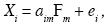
where X is the ith score after it has been standardized to have a mean of zero and a standard deviation of one for all of the m wells; aim is a constant named the factor loading, Fm is the factor value which has mean of zero and standard deviation of one for all the wells, and ei is the part of Xi that is specific to the ith test only.
Thus, the general factor analysis model takes the form
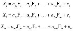
With this model, the total variance of Xi = a2i1 + a2¡2 + ... + a2im + Var(ei); i.e., the variance of the original variable is disseminated through the factors. The correlation between variables is rij = ai1 aj1 + ai2 aj2 + ... + aim ajm . Hence two test scores can only be highly correlated if they have high loadings on the same factor.
In this way, the factor loadings are not unique since each factor is a linear combination of the other factors on the form F* m = dm1 F1 + dm2 F2 +...+ dmm Fm, and are called provisional factors. These provisional factors are transformed through a procedure called factor rotation in order to find new factors that are easier to interpret. Factor rotation can be orthogonal (i.e. Varimax rotation), and the new factors are uncorrelated. Numbers of factors that can be retained depend on the quality and quantity of data and it is expected that a large part of the variance in the original series is accounted for by the factors. It is desirable that the factor loadings for the new factors should be either close to zero or very different from zero. A large (close to 1) positive or negative a¡j means that Xi is determined by Fm to a large extent. When it is the case, Fm explains a large part of the variance in the original variables which means that wells are highly correlated (Manly, 2005). Furthermore, plotting on a map the factor loadings separately for each factor (i.e., ai1 for F1; ai2 for F2; etc.) allows the definition of regions if large values (positive or negative) of ai clustered in the same geographic locality. Hence, the number of regions equaled the number of retained factors. In this case it might be concluded that values of samples in the wells are regionally comparable and come from the same origin. The boundary between the regions could be established by selecting an arbitrary value of ai, but the more close to 1 is this value the more highly correlated are the wells in the region. In the present study groups of wells were produced with a = 0.70 loading contour.
Results
The summary of sample values in Table 1 shows large differences between minimum and maximum values in all the parameters, from the surface to the first 100 m depth, indicating large variability of water quality in the aquifer. A matrix correlation from some arbitrary selected wells (Table 2), indicate that high correlations are common between the wells even though they are long distance apart. Therefore, it was quite conceivable that 135 variables (wells) could be adequately represented by some factor–regions.
Indeed, Table 3 shows that the first three retained factors account for 99% of the total variance of the wells. The variance accounted for by each factor is very high, 38% for Factor 1, 33% for Factor 2, and almost 28% for Factor 3. Highly correlated variables (i.e., those variables with factor loadings a≥0.7 in each factor), sum up 43 for Factor 1, 26 for Factor 2, and 15 for Factor 3 (Table 3 and Fig. 3). Those wells with associated a<0.70 in the three retained factors were considered undefined (not–belonging to any Factor). These variables sum up 47, and they are randomly distributed in the region with numbers (see Fig. 1): 6–8,10, 11, 13–15, 17, 18, 23, 29, 33, 35, 36, 40–43, 46–49, 51, 53, 54, 57, 58, 64, 67, 69, 73, 75, 78, 89–91, 96, 98, 105–108, 111, 118, 128, and 129. Causes of no–definition of these variables seem to be related to localized conditions. Because these wells do not contribute information that elucidates the differences between the areas, they were not considered in subsequent calculations. Considering that in EOF analysis Factor 1 to Factor 3 are uncorrelated common factors (Manly, 2005), the large percentage of the variance explained in each of them indicate a clear distinction between the factors. Also, that all of them are equally important for accounting for the total variance in the original series. Fig. 3 displays the loading contour maps for Factor 1 (Fig. 3a), Factor 2 (Fig. 3b) and Factor 3 (Fig. 3c). A composite map displaying factor loading contours a≥0.7 from the three maps (shading areas) is shown in Fig. 3d. Crosses in Fig. 3d indicate the position of wells monitored in 2003. Note that wells are distributed in the three areas and that each of the areas is geographically well defined: to the east and southeast for Factor 1 ("eastern area"); to the west for Factor 2 ("western area"); and to the center on a northwest–southeast narrow strip for Factor 3 ("central area").
There were few cases with values a>0.7 apart from the main shading area, for example well 94 to the southeast in Factor 2 (Fig. 3b), and wells 132, 125, 127 to the southwest in Factor 3 (Fig. 3c). Because these wells are not defined in the main shading area they were removed from calculations and were considered also as undefined wells.
Constituents from wells that were defined in Factors 1–3 after EOF analysis, were averaged and their respective standard deviations were calculated (Table 4). To verify how well the distinction between the areas is defined in more recently conditions, average values and standard deviations of constituents were also estimated from wells monitored in May 2003 (Table 5), and after locating them in their respective area (see Fig. 3d). Wells associated to each factor were: for Factor 1–eastern area 23–28; for Factor 2–western area 1, 2, 8–17; and for Factor 3–central area 3–7 and 22 (see Fig. 3d). Note, that wells 25 and 26 are located outside of the shading area (Fig. 3d), but still related to the eastern area because they are apart from the other areas.
Discussion
EOF analysis has been used to identify possible sources/ factors that influence the water systems (Simeonov et al., 2003, Méndez–Rodríguez et al., 2008), in which the variables are the characteristics of water quality and the individuals correspond to the monitoring sites (wells). Another application of this method has been recognition of highly correlated elements to delimit regions. In this case factor loadings associated to each variable are plotted on a map and the border between the regions is assigned by selecting an arbitrary factor loading value closed to 1. This application has gained success in hydrometeorology studies (Richman, 1981; Comrie and Glen, 1988; Brito–Castillo et al., 2003) and more recently an extensive review about EOF application in atmospheric sciences has been done (Hannachi et al., 2007). In this work the second approach has been applied. The motivation to do this was to focusing on the highly correlated sites making computations for 12 characteristics of water quality between the wells. It is assumed that if subsurface water is in contact with geologic materials of similar characteristics, then its quality, analyzed from the samples from the wells, should be comparable (i.e., highly correlated). Actually, major–ion chemistry of natural waters can often be explained by the reaction of these waters with rocks or sediments through which they flow (Frape et al., 1984; Hem, 1989; Thomas et al., 1989). On the other way, if the water composition is dissimilar (i.e. correlation between the wells is near zero), then one may assume that water belongs to aquifers with different geologic environments, or the differences in water quality might result from extrinsic man–made factors (Pye and Patrick, 1983). Hence, the discussion below is focusing on demonstrating that highly correlated wells (i.e., wells assigned to the same factor), are explained by similar characteristics of water quality that distinguished them from other non–related to the same factor wells. In other words, this means that the western, central, and eastern areas (Fig. 3) might be distinguished by predominance of different parameters of water quality. Then, the discussion involves more recently measurements from wells located in each of the areas.
In the western area, average values of Na+, K+, E.C., SO42–, Cl–, and TDS (Table 4) are indicative of high salinity, low rainfall (CNA, 1991), and high evaporation (1700 mm/year) (Ortlieb and Pierre, 1981). In this part of the Reserve, evaporation is so high that salt production is a major economic activity. The salt ponds of Guerrero Negro are one of the largest salt fields in the world (S ARH, 1991). This is an area of evaporite deposits, brine pans, and salt flats (Ortlieb and Pierre, 1981) with presence of gypsum beds, halite (Kinsman, 1969; Phleger, 1969), and uncommon mineral, polyhalite (Holser, 1966), which largely explain high concentration of Na+, K+, SO42–, Cl– in groundwater. In this area, 10 out of 26 wells (Fig. 3b) are classified as highly salty (INEGI, 1989). Three of the wells are used for industrial purposes and 18 wells were for domestic and livestock uses. More recently measurements (Table 5) confirmed these results, indicating that ground water in the western area is brackish (Carriker, 1967), with high conductivity and high concentrations of Na+, Cl, SO42–, and TDS compared to the two other areas (Table 5). At present, the wells positioned in the western area are abandoned, but it was possible to confirm that in the past, those wells were of domestic and livestock uses as it was reported (INEGI, 1989).
The eastern area is dominated by bicarbonate ions HCO3– and smaller concentrations of the other dissolved constituents, in comparison to the other two areas (Table 4). Average NO3–N concentrations are a little higher than in the west. The predominance of carbonate alkalinity in groundwater in the eastern area is explained by the reaction of water with subaerial andesitic and basaltic flows, tuff, breccia, agglomerate, and tuffaceous sandstone (Ochoa–Landín et al., 2000). These rocks define a medium–K calc–alkaline suite typical of active continental margins (Sawlan and Smith, 1984) as is the case of Santa Rosalía basin (Ochoa–Landín et al., 2000) in the eastern area.
Values of HCO3– between 50 and 400 mg/L are common in groundwaters (Hem, 1989) as occur in the three areas, and values of Ca2+, Na+, and K+ higher than 15, 6.3, and 2.3 mg/L, respectively, as is observed in the eastern area (Tables 4 and 5) come from mineralized waters common in arid regions (Davis and DeWiest, 1968).
Because of the presence of gypsum deposits in the eastern area (INEGI, 1983; Ochoa–Landín et al., 2000), calcium concentration and the dissociation of HCO3– is high. It is possible to assume that calcium concentration has increased by the presence of sodium and potassium salts (Davis and DeWiest, 1968) through a mechanism known as ion exchange (Foster, 1942), which largely explains the increase in water hardness (Sawyer and McCarty, 1967) in the eastern area. Hardness increased from 289 mg/L, Table 4 in 1983 to very hard (414 mg/L) at present (Table 5).
Groundwater quality of the eastern area differs from that of western and central areas in soluble ammonia (0.2 mg/L, Table 5) which is also the maximum concentration recommended by WHO (1996). Ammonia is formed by the deamination of organic nitrogen – containing compounds and by the hydrolysis of urea (GEMS, 1992). It is easily oxidized to nitrite and nitrate in the presence of sufficient oxygen (nitrification). This constituent by itself has no direct importance for health but might be an important indicator of fecal contamination. Unfortunately, we don't have the analysis to prove that. The 43 wells located here are commonly used for domestic purposes and irrigation (10 wells) and livestock (19). High levels of soluble ammonia in groundwater produce bad taste and odor problems among other aspects (WHO, 1996).
The central area is characterized by nonindurated sediments (alluvium), sand deposits and conglomerates, allowing a high volume flow groundwater in this part of the aquifer (INEGI, 1983). The highest density of agricultural fields occur in this area. Of eleven wells recently monitored in the area (see location of wells in Fig. 3d), four wells are used for irrigation, four wells are used for irrigation and domestic purposes, and three solely for domestic purposes. Because the use of agricultural chemicals (mainly nitrate fertilizers) (Matson et al., 1997), this area has the highest average concentrations of nitrates in groundwater now (Table 5), as it had in the past (Table 4) compared to the other areas. In 1983, central area water was very hard (hardness = 647 mg/L) dominated by calcium (75.8 mg/l) and magnesium (106.9 mg/L) (Table 4) (INEGI, 1983). These average concentrations were estimated from data reported by INEGI (1983), but we found that average hardness and calcium and magnesium were 162, 27 and 23 mg/L, respectively (Table 5), which is more credible than previous values because magnesium is generally found in lower concentrations than calcium (Davis and DeWiest, 1968) and also, because the largest concentration of magnesium (57.3 mg/L) was in the western area (Table 5) which matches with the presence of magnesite and dolomite encountered in sedimentary rocks in that area (Padilla–Arredondo et al., 1991). Average salinity in groundwater in the central area is 0.4 psu, a value that is close to the 0.5 psu limit for brackish water (Carriker, 1967). The high salinity suggests salt water intrusion to the aquifer from the west presumably caused by large groundwater withdrawals for irrigation (Bear et al., 1999). The advance of saltwater from the west has affected the position of salt water–fresh water transition degrading the quality of water for domestic uses in the west as has been mentioned previously. Large withdrawals from the Vizcaino aquifer decrease the volume of fresh water available and result in storage deficit (Matson, 1997). Most water from precipitation that infiltrates does not become recharge. Instead, it is stored in the soil zone and is eventually returned to the atmosphere by evaporation and plant transpiration (Alley et al., 2002). Values published (DOF, 2003) indicate that average annual groundwater recharge in Vizcaino aquifer is negative at 1.7 x 10⁶ m3.
Conclusions
The National Water Commission of Mexico (CNA) has considered the aquifer located in the Reserve as one water body. We applied Varimax rotated EOF analysis to data of 135 wells using the information of 12 parameters of water quality; the Factors 1–3 retained in the analysis, were compared to the composition of the geologic deposits present. The results of this comparative analysis indicate that water quality in this aquifer within the Reserve is differentiated into eastern area, western area, and central area. Thus the EOF analysis proves to be an excellent tool for this kind of investigations and this technique might be applied in other areas with available groundwater chemical data. Results indicate that the eastern area is characterized by average high concentration of bicarbonate ions caused by the reactions of water with rocks that define a medium–K calc–alkaline suite. The western area is characterized by average high concentrations of Na+, K+, SO42–, Cl– and TDS, a result from the dissolution of gypsum, halite and polyhalite minerals. The groundwater in the central area shows high concentrations of soluble nitrates, a product of agricultural fertilizer. Because of high withdrawals in the central area, the advance of saltwater from the west is already evident. The results of this study can be useful to stakeholders and the public interested in a better groundwater management of this aquifer.
Acknowledgements
We thank the director of Conservation and Environmental Planning Program of CIBNOR for his support. This study received financial support of the following projects: CONANP 727–0, CONACYT M0029–2006–1–42027, J50757, and CIBNOR PC2.3., and PC 1.3. The staff editor at CIBNOR improved the English text.
Bibliography
Alley, W. M., R. W. Healy, J. W. LaBaugh and T. E. Reilly, 2002. Flow and Storage in Groundwater Systems. Science 296, 1985–1990. [ Links ]
APHA, 1992. Standard Methods for Examination of Water and Wastewater, 18th Ed. American Public Health Association, Washington DC. [ Links ]
Bear J, A. H. – D. Cheng, S. Soreck, D. Ouazar and I. Herrera, 1999. In Bear J, Cheng AH –D, Soreck S, Ouazar D, Herrera I (ed.), Seawater Intrusion in Coastal Aquifers. Concepts, Methods, and Practices, Kluwer, Dordrecht, Neherlads. [ Links ]
Brito–Castillo, L., A. V. Douglas, A. Leyva–Contreras, D. Lluch–Belda, 2003. The effect of large–scale circulation on precipitation and streamflow in the Gulf of California continental watershed, Int. J. Climatol. 23, 751–768. [ Links ]
Carriker, M. E., 1967. Estuaries, p. 442, In Lauff GH (ed.), Publication 83, American Association for the Advancement of Science, Washington, D.C. [ Links ]
CNA, 1991. Isoyetas normales anuales de la República Mexicana. Período 1930–1990. Regiones hidrológicas 2 Baja California Centro Oeste (Vizcaíno); 5 Baja California Centro Este (Santa Rosalía), Map 2, Comisión Nacional del Agua, COINPRO, S. A. de C. V., D. F., México. [ Links ]
Comrie, A. C. and E. C. Glenn, 1998. Principal components–based regionalization of precipitation regimes across the southwest United States and northern Mexico, with an application to monsoon precipitation variability, Climate Res. 10, 201–215. [ Links ]
Davis, S. N., R. J. M. De Wiest, 1968. Hydrogeology, John Wiley & Sons, Inc., New York. [ Links ]
Dirección General de Geografía, 1983. Geología de la República Mexicana. D. F. México, 79 pp. [ Links ]
DOF, 2003. Diario Oficial de la Federación, vienes 1 de enero del 2003, Segunda sección, D. F., México. [ Links ]
Foster, M. D., 1942. Base exchange and sulfate reduction in salty ground waters along Atlantic and Gulf coasts, Am. Assoc. Petroleum Geologists Bull. 26, 838–851. [ Links ]
Frape, S. K., P. Fritz, R. H. McNutt, 1984. Water–rock interaction and chemistry of groundwaters from the Canadian Shield. Geochim. Cosmochim. Acta 48, 1617–1627. [ Links ]
García,E., 1988. Modificaciones al sistema de clasificación climática de Koppen para adaptarlo a las condiciones de la República Mexicana, 222 pp, Offset Larios, México. [ Links ]
Gastil, R. G., R. P. Philips and E. P. Allison, 1975. Reconnaissance geology of the State of Baja California. Geol. Soc. of America Memoir 140, 170 p. [ Links ]
GEMS, 1992. Global environment monitoring system. UNEP/WHO/UNESCO/WMO programme on global water quality monitoring and assessment. GMES/ Water operational guide. Third edition, GEMS/W.92.1. Geneva, Switzerland. [ Links ]
Hannachi, A., I. T. Jollife and D. B. Stephenson, 2007. Empirical orthogonal functions and related techniques in atmospheric sciences. A review. Int. J. Climatol. 27, 1119–1152. [ Links ]
Hausback, B. P., 1984. Cenozoic Volcanism and Tectonic Evolution of Baja California Sur, p. 219–236, In Frizzell VA Jr. (ed.), Geology of the Baja California Peninsula, vol. 39, Society of Economic Paelontologic and Mineralogist, Pacific Section, Los Angeles CA. [ Links ]
Hem, J. D., 1989. Study and interpretation of the chemical characteristics of natural water, Water–Supply Paper 2254, US Geological Survey, Reston, VA. [ Links ]
Holser, W. T., 1966. Diagenetic polyhalite in recent salt from Baja California, American Mineralogist 51, 99–109. [ Links ]
INEGI, 1983. Instituto Nacional de Estadística, Geografía e Informática. Carta hidrológica de aguas subterráneas, esc. 1: 250,000, Map G12–1 Santa Rosalía, México. [ Links ]
INEGI, 1989. Instituto Nacional de Estadística, Geografía e Informática. Carta hidrológica de aguas subterráneas, esc. 1: 250,000, Map G11–3 Guerrero Negro, México. [ Links ]
INEGI, 1996. Instituto Nacional de Estadística, Geografía e Informática. Estudio Hidrológico del Estado de Baja California Sur. Aguascalientes, Ags. Méx. 205 p. [ Links ]
Kinsman, D. J,. 1969. Modes of formation, sedimentary associations and diagnostic features of shallow–water and supratidal evaporates. American Association Petroleum Geologists Bulletin 53, 830–840. [ Links ]
López–Ramos, E., 1980. Geología de México. UNAM., México, D. F. Ed. Escolar tomo II. 453 pp. [ Links ]
Lozano, F., 1976. Evaluación petrolífera de la península de Baja California, Boletín de la Asociación Mexicana de Geólogos Petroleros 27, 106–303. [ Links ]
Lugo–Hubp, J., 1990. El relieve de la República Mexicana, Revista Mexicana de Ciencias Geológicas 9, 82–111 (free available at http://satori.geociencias.unam.mx/TOC.htm). [ Links ]
Manly, B. F. J., 2005. Multivariate Statistical Methods. A Primer, 214 pp., Chapman & Hall/CRC, London. [ Links ]
Mc. Lean, H., B. P. Hausback and J. H. Knapp, 1987. The Geology of West–Central Baja California Sur, México, U.S. Geological Survey Bulletin 1579, 16. [ Links ]
Matson, P. A., W. J. Parton, A. G. Power and M. J. Swift, 1997. Agricultural Intensification and Ecosystem Properties, Science 277, 504–509. [ Links ]
Méndez–Rodríguez, L. C., S. C. Gardner, L. Brito–Castillo, B. Acosta–Vargas, J. Wurl and S. T. Alvarez–Castañeda, 2008. Distinguishing the Hydrochemistry of Tw Hydrological Basins in Northern Mexico Using Factor Analysis. Water Quality Journal of Canada, 43(2/3), 111–119. [ Links ]
Mina, F., 1957. Bosquejo geológico del territorio sur de la Baja California, p. 139–267. In Benavides L (ed.), Boletín de la Asociación Mexicana de Geólogos Petroleros, vol. IX, no 3 and 4, D.F., México. [ Links ]
Montgomery, D. R. and M. Manga, 2003. Streamflow and Water Well Responses to Earthquakes, Science 300, 2047–2049. [ Links ]
Müller, R. D., M. Sdrolias, C. Gaina, B. Steinberger and Ch. Heine, 2008. Long–Term Sea Level Fluctuations Driven by Ocean Basin Dynamics. Science 319, 1357–1362. DOI: 10.1126/Science. 1151540. [ Links ]
Ochoa–Landín, L., J. Ruiz, T. Calmus, E. Pérez–Segura and F. Escandón, 2000. Sedimentology and Stratigraphy of the Upper Miocene El Boleo Formation, Santa Rosalía, Baja California, México, Revista Mexicana de Ciencias Geológicas, 17, 83–96 (free available at http://satori.geociencias.unam.mx/TOC.htm). [ Links ]
Ortlieb, L. and C. Pierre, 1981. Génesis evaporítica en tres áreas supralitorales de Baja California; contextos sedimentarios y procesos actuales, Revista Mexicana de Ciencias Geológicas 5, 94–116 (free available at http://satori.geociencias.unam.mx/TOC.htm). [ Links ]
Padilla–Arredondo, G., S. Pedrín–Avilés and E. Troyo–Diéguez. 1991, Geología, In La Reserva de la Biosfera El Vizcaíno en la Península de Baja California by Ortega A. and L. Arriaga (eds.) pp. 71–93, Centro de Investigaciones Biológicas de Baja California Sur AC, B. C. S., México. [ Links ]
PEMEX, 1976. Prospección Geológica en Baja California. Reporte Técnico de la Gerencia de Exploración de Petroleos Mexicanos, México, D. F. [ Links ]
Phleger, F. B., 1969. A modern evaporite deposit in Mexico, American Association Petroleum Geologists Bulletin 53, 824–829. [ Links ]
Pye VI and R. Patrick, 1983. Ground Water Contamination in the United States, Science 221, 713–718. [ Links ]
Richman, M. B., 1981. Obliquely rotated principal components: an improved meteorological typing technique?, J. Appl. Meteorol. 20, 1145–1159. [ Links ]
SARH, 1991. Sinopsis geohidrológica del estado de Baja California Sur, 85 pp., Secretaría de Agricultura y Recursos Hidráulicos, Talleres de Sistemas Gráficos E., S.A. de C.V., D.F., México. [ Links ]
Sawlan, M. G. and J. H. Smith, 1984. Petrologic Characteristics, Age and Tectonic Setting of Neogene Volcanic Rocks in Northern Baja California Sur, Mexico, p. 237–251. In Frizzell VA Jr (ed.), Geology of the Baja California Peninsula, vol. 39, Society of Economic Paelontologic and Mineralogist, Pacific Section, Los Angeles CA. [ Links ]
Sawyer, C. N. and P. L. McCarty, 1967. Chemistry for Sanity Engineers, 2nd ed., McGraw–Hill Book Co, NewYork. [ Links ]
Shreve, F., 1936. The plant Life of the Sonoran Desert, The Scientific Monthly 42, 195–213. [ Links ]
Simeonov, V., J. A. Stratis, C. Samara, G. Zachariadis, D. Voutsa, A. Anthemidis, M. Sofoniou and Th. Kouimtzis, 2003. Assesment of the Surface Water Quality in Northern Greece, Water Research 37, 4119–4124. [ Links ]
Thomas, J. M., A. H. Welch and A. M. Preissler, 1989. Geochemical Evolution of Groundwater in Smith Creek Valley– a Hydrologically Closed Basin in Central Nevada, USA, Applied Geochem. 4, 493–510. [ Links ]
WHO, 1996. Guidelines for Drinking–Water Quality. Health criteria and other supporting information, 2nd ed., World Health Organization, Geneva. [ Links ]

