


 nova página do texto(beta)
 Inglês (pdf)
 Artigo em XML
 Referências do artigo
 Enviar este artigo por email
 Citado por SciELO
  Similares em
SciELO
Similares em
SciELO 
 Permalink
Introduction
During mass measurement of weights in the air, their density or volume must be known, to be able to calculate the corresponding air buoyancy correction (Jones and Schoonover, 2002; Malengo and Bich, 2012; Schwartz, 2000). In the International Organization of Legal Metrology [OIML] recommendation R 111-1 (2004), six different methods for the determination of the density of weights are described, including immersion in liquids, a databased method, and a geometric measurement method. Among these methods, the hydrostatic weighing method is the most accurate (Jian et al., 2012), and even the one used during comparisons concerning the determination of the volume of weights between National Metrology Institutes (Becerra et al., 2015).
However, the hydrostatic weighing method is not simple to implement and consumes a considerable amount of time when the volumes of a series of weights need to be determined, due mainly to the times of drying and tempering (Kobata et al., 2004; Malengo and Bich, 2012). So, when the immersion of the weight in a liquid is not an option, it is called Method E, that is, the volume determination of the weights by geometric measurement became a good option. Even though risk of scratching the surface is present during the geometric measurement of the weight, the restriction of the method on class E and F weights is advised (Myklebust et al., 1997; OIML, 2004).
Of course, the six methods listed in OIML (2004) are not the only possibilities for the determination of the volume of weights. Clarkson et al. (2001) and Malengo and Bich (2012) have reported on the weighing in the air with different densities. In that method, the use of mass comparators inside sealed chambers is required, so this kind of measurement of the volume of weights is almost exclusive for NMIs. Another method was first proposed and then widely studied in Asia, by Ueki et al. (1999), Kobata et al. (2004), Ueki et al. (2007), and Jian et al. (2012) among others. This method uses a device called acoustic volumeter, yet it is not explicitly designed for the measurement of standard weights, but rather any solid object. Even when the method is very accurate, it requires at least one (preferably two) reference weight with a known volume and similar shape of that one under volume determination.
Finally, in another work, a first attempt to use Method E to determine the volume of OIML class E and F weights (OIML, 2004) using an optical comparator was done (Purata et al., 2015). In that study, the risk of scratching the surface of weights was eliminated, with the replacement of the Vernier caliper with the optical comparator. This technique was also already used in reference weights of pressure balances (Purata-Sifuentes et al., 2017). However, as pointed in OIML (2004) the biggest contributor to the volume measurement uncertainty still was the deviation of the real weight shape from the mathematical model. Purata et al. (2015) also realized that the shape of the weights could vary from one set of weights to another (different or same manufacturer), or there could be variation between weights of the same set (same manufacturer). This could be explained because some of the class E2 weight sets still in use for calibration are even twenty years old, when the manufacturing processes were not as controlled and advanced as nowadays.
In this work, an improved mathematical model for the calculation of the volume of OIML (2004) weights through Method E was developed. Violations of the constraints from the proposed shape in OIML (2004) Method E, specifically in the knob and in the ring, are addressed and corrected during the new model development. An increased possibility to improve adjustment of the proposed mathematical model to the real shape of the weights was observed when both models were compared, the current OIML (2004) one, and the proposed in this work.
Geometric measurement of weights
Density Test Method E in OIML (2004) assumes that weight is an assembly of four simple geometric forms. Therefore, the weight volume (Vweight) becomes the algebraic sum of the volumes of the four sections: the knob A, the ring B, the body C, and the recess D (Figure 1, without recess).
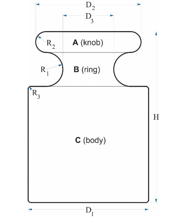
Source: based on Figure B.8 in OIML (2004).
Figure 1 The four different sections for weight volume determination by geometric measurement
An equation (5) is the algebraic sum of the four volume sections. Equation (4) is elementary, just the formula of a truncated circular cone; hence, it will not be addressed in this work anymore. Now, even though equations (3) to (1) are not difficult to understand, deduction of equation (1), i.e., the volume formula of the knob, is shown as an example of how to proceed, and because the intermediate equations will serve later.
Derivation of equation (1)
The knob must be divided into two parts. The first one is a straight circular cylinder with a radius equal to (D2/2 - R2) and a height equal to 2R2 (Figure 1). The second par is a solid of revolution with the center in the symmetry axis of the weight. The cross-section of this solid of revolution is a semicircle with a radius equal to R2, and its centroid is located on its symmetry axis, at 4R2/3π from the straight edge of the semicircle. The volume of a solid of revolution is the product of the cross-section area times the circumference followed by the centroid during the revolution (Beer et al., 2016). Therefore, the equations preceding equation (1) are:
Equation (7) could easily be rearranged to become equation (1). Equations (2) and (3) could be developed following a similar strategy, i.e., using a straight circular cylinder combined with a solid of revolution. There is only one difference to be considered in the case of section B of the weight: the volume of the solid of revolution, if generated with a semicircle, must be subtracted from the base cylinder volume instead of added to it.
Assessment of the current mathematical model
Equation (1), published in OIML (2004), assumes that the knob ends in a semicircle shape, as was considered during the development of equations (6) and (7) that lead to equation (1). The same assumption applies for the volume determination of the ring section, VB : it is necessary to assume that the shape of the edge of the ring is an outward concavity semicircle, to be able to deduce equation (2). However, to support these assumptions, the following relation between diameters and radii in the knob and the ring would have to be met (Figure 1):
Annex A of OIML (2004) includes examples of dimensions for cylindrical weights with nominal values ranging from 1 g to 20 kg. None of the examples result in compliance with equation (8). For all the example data sets published in OIML (2004), the left-side of equation (8) is smaller than the right-side. The current mathematical model of OIML (2004) Method E implies an important deviation from the current shapes of the weights, specifically in the knob and the ring. Of course, in the real dimensions of weights, D3 will always be smaller than D2, so the problem with the current mathematical model seems to be the assumption that both sections, the knob, and the ring, end in semicircles. A way to solve that, is to consider the edges of the knob and the ring just as circular sectors, instead of semicircles (Figure 2).
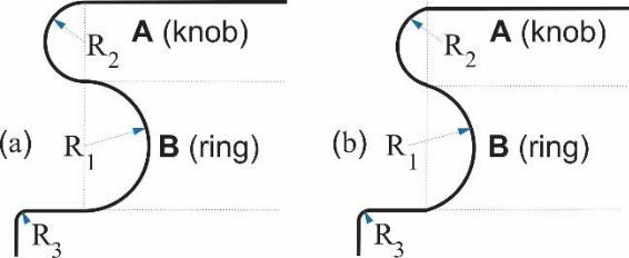
Source: elaborated by the author.
Figure 2 Profiles of weight with edges of the knob and the ring modeled as (a) semicircles, and (b) circular sectors
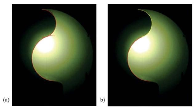
Figure 3 shows a picture of real OIML R 111-1 weights measured with an optical comparator. The edges of both sections, the knob, and the ring are best fitted with circular sectors (b) than with semicircles (a). Figure 3a has two red semicircles: one in the knob from 90° to 270°, and another in the ring from 270° to 450°, clockwise. On the other hand, Figure 3b has a yellow circular sector that goes from 90° to 255°, whereas the ring sector (red) in the same figure goes from 270° to 428°, also clockwise. The excess on both contours of Figure 3a is notorious.
An improved mathematical model
The edges of the knob and the ring could be modeled more accurately as circular sectors in the way shown in Figure 4. The idea considers the possibility that the knob or the ring (or even both) could not be symmetrical around the horizontal that passes through the origin of R2 or R1, respectively. These assumptions imply the following relation between diameters and radii in the knob and the ring (Figures 2b and 4):
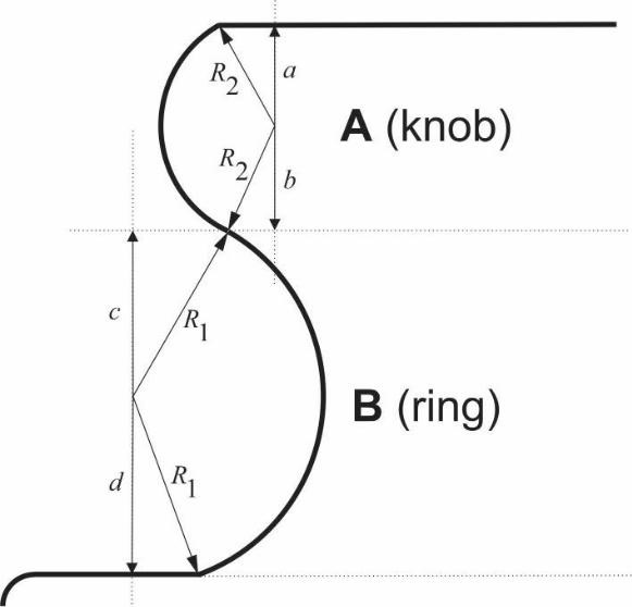
Source: elaborated by the author.
Figure 4 Proposed profile model for the edge of the knob and the ring of the weight
Equation (9) can be satisfied for all the included sets of dimensions for cylindrical weights with nominal values ranging from 1 g to 20 kg, published in Annex A of OIML (2004), provided at least one of the following restrictions is met: c < R1 or b < R2.
If the procedure described before to compute the volume is followed, it is possible to develop new equations for the volume of the knob, VA, that will substitute equation (1), and for the volume of the ring, VB, that will substitute equation (2) during weight volume calculation.
A new equation for the knob
The knob must be divided into two parts. The first one is a straight circular cylinder with a radius equal to [D2 /2 - R2], but this time its height equals [a + b] (Figure 1, and knob section of Figure 4). The second part is a solid of revolution with the center in the symmetry axis of the weight, whose cross-section area is the cut semicircle with a radius equal to R2 shown in the knob section of Figure 4. Calculation of that cross-section area is straight-forward by integration.
Integration could also be used to locate the centroid of the cut semicircle knob,
The volume of a solid of revolution is the product of its cross-section area times the circumference followed by its centroid during the revolution (Beer et al., 2016). Therefore, the new equation that substitutes equation (1), when weights with cut semicircle knob are being modeled is:
Is easy to see that if a = b = R2, that is when the knob section of Figure 4 becomes a semicircle, equation (12) reduces to equation (7), and from it to equation (1).
A new equation for the ring
The ring also needs to be divided into two parts, but this time a subtraction approach is used. The first part is a straight circular cylinder with a radius equal to [D3 /2 + R1], and its height equals [c + d] (Figure 1, and ring section of Figure 4). The second part, whose volume must be subtracted from that of the first part, is a solid of revolution with the center in the symmetry axis of the weight, which cross-section area is the cut semicircle with a radius equal to R1 shown in the ring section of Figure 4. Calculation approach of that cross-section area (Aring, below) is the same as for equation (10), so
Location of the centroid of the cut semicircle ring,
Finally, the new equation that substitutes equation (2), when weights with cut semicircle ring are being modeled is:
It can also be shown by simple substitution that equation (15) reduces to equation (2) when c = d = R1, that is when the ring section of Figure 4 becomes a semicircle.
The new mathematical model for Density Test Method E in OIML (2004) is described by equations (12), (15), (3), (4) and (5). It is important to note that it is unnecessary to increase the rigorousness of equations (3) and (4) given the negligible contribution it will make to the weight volume measurement uncertainty.
Results and discussion
Ueki et al. (1999), published data from geometrical measurements of standard weights with nominal values ranging from 1 g to 10 kg (see Table 1). The main set of weights measured was manufactured with the intention of having the volume calculated for weight with a reference density of 8 000 kg/m3. A Vernier caliper and a height gage were used to do the measurements. A more accurate value of the volume of each weight, measured by the hydrostatic weighing method, was also reported.
Table 1 Dimensional parameters used for the comparison of the proposed model vs. the current one
| Weight | Dimensional characteristics / mm | ||||||
|---|---|---|---|---|---|---|---|
| D1 | D2 | D3 | R1 | R2 | R3 | H | |
| 10 kg | 99.7 | 90.0 | 58.0 | 15 | 8.5 | 3 | 183.0 |
| 5 kg | 79.6 | 72.0 | 46.1 | 12 | 6.5 | 2 | 144.0 |
| 2 kg | 59.6 | 54.1 | 36.1 | 9 | 5 | 2 | 102.45 |
| 1 kg | 47.9 | 42.9 | 27.0 | 7 | 4 | 2 | 80.80 |
| 500 g | 37.8 | 33.9 | 22.1 | 5.5 | 3 | 1.5 | 64.10 |
| 200 g | 28.0 | 25.0 | 16.1 | 4 | 2.25 | 1.5 | 47.10 |
| 100 g | 21.8 | 19.9 | 13.2 | 3.5 | 2 | 1 | 38.60 |
| 50 g | 17.9 | 15.8 | 10.2 | 2.5 | 1.5 | 1 | 29.40 |
| 20 g | 12.7 | 11.3 | 7.8 | 1.8 | 1 | 0.5 | 22.80 |
| 10 g | 9.8 | 8.9 | 6.1 | 1.5 | 0.8 | 0.5 | 18.75 |
| 5 g | 7.8 | 6.9 | 4.2 | 1.25 | 0.7 | 0.5 | 15.35 |
| 2 g | 5.8 | 5.2 | 3.2 | 0.9 | 0.5 | 0.5 | 11.10 |
| 1 g | 5.8 | 5.3 | 3.2 | 0.9 | 0.5 | 0.5 | 6.30 |
Source: Ueki et al. (1999).
The new mathematical model, equations (12), (15), (3), (4), and (5), were compared to the current model, equations (1), (2), (3), (4), and (5), using the values for the diameters, radii and height published by Ueki et al. (1999) (Table 1). It is important to remember that the new model implies the use of an optical comparator to do all the geometrical measurements, since the new model parameters: a, b, c, and d, cannot be measured with a Vernier caliper. However, the use of the measurements made by Ueki et al. (1999) could be used here only for comparison purposes.
Assessment of the new model error
Table 2 contains the results of both mathematical models and the reference hydrostatic weighing values. Both sides of the geometrical constraints of each model, equations (8) and (9) are also included. In this case, the values assumed for the new model additional parameters (Figure 4) were: a = R2, b = 0.975 R2, c = 0.925 R1, and d = R1, for all the weights (first column in Table 2). These values correspond to the rounded values obtained with the geometry of the real weight shown in Figure 3b. It is important to remark that the values for the parameters a, b, c, and d, could be different for every weight (and they probably must be). But validity is not lost if they are taken as the same for all the weight values, just for the assessment of the new model.
Table 2 Volume determination by the current OIML model, the hydrostatic weighing method and the proposed new model
| Weight nominal value | l.s. Eqs. (8, 9) | r.s. Eq (8) | VOIML / cm3 | VHW / cm3 | VNewModel / cm3 | r.s. Eq (9) |
|---|---|---|---|---|---|---|
| 10 kg | 90.0 | 105 | 1259.19 | 1255.48 | 1252.53 | 89.8 |
| 5 kg | 72.0 | 83.1 | 631.10 | 627.61 | 627.73 | 71.1 |
| 2 kg | 54.1 | 64.1 | 251.43 | 251.13 | 249.93 | 55.0 |
| 1 kg | 42.9 | 49 | 126.389 | 125.591 | 125.708 | 41.9 |
| 500 g | 33.9 | 39.1 | 62.985 | 62.806 | 62.639 | 33.6 |
| 200 g | 25.0 | 28.6 | 25.282 | 25.117 | 25.147 | 24.6 |
| 100 g | 19.9 | 24.2 | 12.616 | 12.570 | 12.536 | 20.7 |
| 50 g | 15.8 | 18.2 | 6.408 | 6.285 | 6.374 | 15.6 |
| 20 g | 11.3 | 13.4 | 2.570 | 2.514 | 2.557 | 11.6 |
| 10 g | 8.9 | 10.7 | 1.265 | 1.257 | 1.257 | 9.2 |
| 5 g | 6.9 | 8.1 | 0.637 | 0.629 | 0.634 | 6.8 |
| 2 g | 5.2 | 6 | 0.255 | 0.252 | 0.254 | 5.1 |
| 1 g | 5.3 | 6 | 0.129 | 0.126 | 0.128 | 5.1 |
l.s. = left side; r.s. = right side; VOIML = volume by current model; VNewModel = volume by new model; VHW = volume by hydrostatic weighing.
Source: elaborated by the author.
The third column of Table 2 contains the values of the right side of equation (8) obtained when the parameter values of Table 1 are used with the current model of OIML (2004). The geometrical constraint for the current model, equation (8), is not satisfied for any of its left and right side values (second and third columns in Table 2). On the other side, the same parameter values plus the additional four stated at the beginning of this section yields nine of thirteen rows in Table 2 with compliance of equation (9), that is, the right side of equation (9) is lower than D2, which is the left side of both equations (8) and (9).
Now, the volume calculated with the new model, VNew-Model, could produce a closer agreement with the more accurately measured volume value by the hydrostatic weighing method, VHW, than the obtained with the current model, VOIML (see columns 4, 5, and 6, in Table 2). Figure 5 shows a semi-logarithmic scale the absolute differences between the hydrostatic weighing volume and the two geometric models for the thirteen weight values of Table 2. Only for the 2 kg nominal value, the current model had more agreement with the hydrostatic weighing value.

D- OIML = ABS(VOIML - VHW); D-NewModel = ABS(VNewModel - VHW). Source: elaborated by the author.
Figure 5 Differences against hydrostatic weighing volume for the current model and the proposed new model. The x-axis is a logarithmic scale
An interesting question is whether the improvement achieved with the new model is statistically significant. This can be carried out by means of a hypothesis test in which the thirteen pairs of differences shown in Figure 5, that is, D- OIML and D-NewModel, are evaluated regarding their statistical significative difference.
The Mann-Whitney-Wilcoxon Test (Mann and Whitney, 1947) determines if the data of two samples come from different populations considering that the samples do not affect each other; thanks to this test we can determine if the data come or not from the same distribution without having to assume that this distribution is normal. The test is performed in R, finding that the p-value with the data of D- OIML and D-NewModel is p = 0.259. The null hypothesis of the test considers that the data come from the same distribution. Considering that the confidence is 95%, we require that the p-value be less than 0.05 in order to discard the null hypothesis and determine how significantly the data come from different populations. So, the Mann-Whitney-Wilcoxon test did not find that the data come from two significantly different populations.
However, the standard deviation and the interquartile range of D-OIML are 1.312 and 0.292, respectively, whereas for the D-NewModel, these two values are 0.840 for the standard deviation and 0.115 for the interquartile range. Hence, there is evidence to indicate that the proposed method is better because the dispersion of the differences between the more accurate hydrostatic weighing method and the proposed geometrical method is lower.
Assessment of the new model uncertainty
Because the Test Method E in OIML (2004) states the use of a Vernier caliper for the dimensional measurements of the parameters, and the new model implies the use of an optical comparator, which has a smaller resolution by one order of magnitude (Dotson, 2016), the uncertainties comparison with the data taken from Ueki et al. (1999) is strictly not possible.
A simplified comparison of uncertainties, using the data from Ueki et al. (1999), through Monte Carlo simulation (Chew and Walczyk, 2012) of both geometrical models, could be done if the values taken by the new model parameters turn out to be: a = 0.995 * R2, b = 0.975 * R2, c = 0.925 * R1, and d = 0.995 * R1. Only a and d values changed from the used in section 4.1, and this is so that the random dispersion during the Monte Carlo uncertainty estimation does not lead to undefined operations in equations (12) and (15). Table 3 contains the combined standard uncertainties (uc…) obtained for both models with a Monte Carlo simulation with 104 trials (Chew and Walczyk, 2012). Only results for 500 g and 1 kg central nominal values were simulated, and normal distributions were assumed for all the parameters. The standard deviations assumed for the parameters, based on (ref#1, year#1) are: (SDD1 = 0.001, SDD2 = 0.007, SDD3 = 0.005, SDR1 = SDR2 = SDa = SDb = SDc = SDd = 0.002 5, SDR3 = 0.013, and SDH = 0.005) mm.
Table 3 Inputs and results in the Monte Carlo uncertainty estimation
| Weight | VOIML / cm3 | uc-OIML (cm3) | VNewModel / cm3 | uc-NewModel (cm3) | VHW / cm3 |
|---|---|---|---|---|---|
| 1 kg | 126.389 | 0.013 1 | 125.708 | 0.018 2 | 125.591 |
| 500 g | 62.985 | 0.008 0 | 62.639 | 0.011 6 | 62.806 |
Source: elaborated by the author.
The new model has bigger uncertainties than the current OIML (2004) model, but both of them have the same effect regarding the VHW value shown in Table 3, i.e., for one nominal weight the discrepancy between the values of VOIML±uc-OIML or VNewModel± uc-NewModel against the VHW value are significant (Taylor, 1997). That is, the VHW values are not within the uncertainty of the current model or that of the new model. However, it is important to note that the closest possible value of the volume with the current model is more distant from the hydrostatic weighing volume than the furthest possible value obtained with the new model.
Conclusions
An improved mathematical model for the knob and the ring sections of OIML R 111-1 weights was developed. The model is based on the use of solids of revolution and centroids formulae and allows a better adjustment to the actual shape of weights. The new model implies the use of an optical comparator to obtain the values of all the dimensional characteristics from Figs. 1 and 5. An additional advantage of using an optical comparator is that geometric characterization of standard weight classes E and F becomes possible since the contact of the surface of the weights during the measurement is avoided (Purata et al., 2015).
The new mathematical model: equations (12), (15), (3), (4) and (5), is a more comprehensive and more versatile one than the current model from OIML (2004), because the new model covers all the range of circular sectors physically possible that could have the edges of the knob and ring; hence, it is possible to model the knob as a semicircle and the ring as a cut semicircle, or vice versa. Also noteworthy is that equation (9) can be satisfied.
The assessment of the new model with previously published geometrical measurements was successful because closer values to the hydrostatic weighing method values were obtained compared to the current OIML model. However, it is important to note that the difference between the volumes calculated with the current OIML model and the volumes calculated with the new model are not statistically significant. The new model, however, showed less dispersion in its different values against the more accurate hydrostatic weighing method. Also, even when a simplified Monte Carlo uncertainty estimation was done, and shows slightly bigger uncertainties for the new model vs. the current one, the uncertainties were not significant.
An important sequel of this work will be the experimental phase, where all the diameters, radii, height, and additional new model four parameters must be measured with an optical comparator. The measurements will be used to show the differences between Test Method E and the new model presented here, while the hydrostatic immersion method could be used as a more accurate reference.
However, the main contributor to the uncertainty of the Test Method E, even with the new mathematical model and the use of an optical comparator, remains to be the difference between the geometry of Figures 1 and 4 and the actual shape of the weight.

