


 texto em
  Inglês (pdf)
 Artigo em XML
 Referências do artigo
 Enviar este artigo por email
 Citado por SciELO
  Similares em
SciELO
Similares em
SciELO 
 Permalink
Introduction
A digital elevation model (DEM) is the graphical representation of databases containing a numerical format of terrain elevations. A DEM shows, in a simplified and numerical way, the geometry of a part of the terrain surface (Mena-Frau, Molina-Pino, Ormazábal-Rojas, & Morales-Hernández, 2011), which can be represented by a set of values indicating points on the surface, and its geographical location is defined by X (longitude), Y (latitude) and Z (altitude) coordinates. It has been agreed that these points are regularly spaced and distributed according to a pattern that, in general, is located in a geographical projection such as the Universal Transverse Mercator (UTM) (Zhoua & Chenb, 2011).
The techniques to carry out topographic surveys with less error are the total station (TS) and GPS RTK; the development of unmanned aerial vehicles (UAV) have enriched the traditional techniques to improve them; this because they generate greater detail of the surface from images or videos taken during the flight. The evolution of computer systems, technological advances in UAV systems and strategies for processing large volumes of data promote research and application (Escalante-Torrado, Cáceres-Jiménez,& Porras-Díaz, 2016). The increasingly recurrent use of UAVs has diversified their application (Colomina & Molina, 2014); however, the basic products generated are images and videos (Ojeda-Bustamante et al., 2016). In this study, their application is focused on the processing needed to obtain orthomosaics and DEMs from photographic images obtained with an airborne camera.
The applications of DEMs obtained from UAVs are diverse, some of which are the generation of terrain models with topographic use (Liu, Liu, Zou, Wang, & Liu, 2012) and surface models in coastal areas (Long et al., 2016), used in agriculture (Mesas-Carrascosa et al, 2015), in forest engineering (Leduc & Knudby, 2018) and archaeology (Toschi et al., 2015), landslide studies (Permata et al., 2016), and monitoring of mine extraction (Wang et al., 2014), of disaster areas (Bendea et al., 2008), and infrastructure damage (Vázquez-Paulino& Backhoff-Pohls, 2017). The objective of this study was to evaluate the technical and operational feasibility of generating DEMs from images obtained with a camera transported in a UAV, and from topographic surveys with TS, as a direct measurement method, and with a geographic positioning system (GPS RTK). Survey errors were compared and evaluated using statistical indicators to clarify advantages and disadvantages.
Materials and methods
Description of the study area
MDEs were carried out on a plot located at the Colegio de Postgraduados, Campus Montecillo, Texcoco, Estado de México, with an area of 1.4 ha (Figure 1 and 2). The equipment used for the topographic surveys were: TS (CST Berger CST305R), GPS RTK (Sokkia GRX1) and camera for the UAV (Phantom 4 pro) (Table 1).
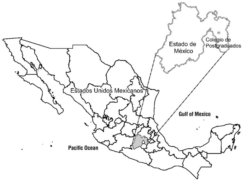
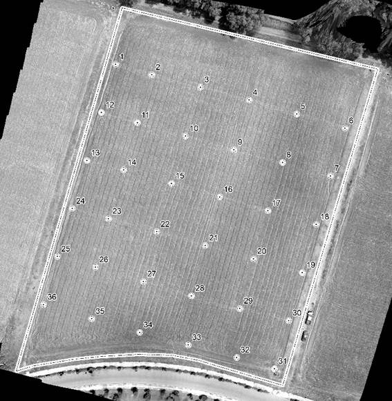
Table 1. Specifications of the topographic equipment.
| Total station | GPS RTK | Unmanned aerial vehicle camera |
|---|---|---|
| Brand: CST Berger CST305R Optical image 30 X magnification 45 mm lens opening 152 mm telescope length 1º 30’ field of vision 1.3 m minimum approach: 5” accuracy 1”/5” direct angular reading Angle measurement: photoelectric detection Measuring range: 1 prism at 3 000 m Measuring range without prism: 200 m Prism accuracy ±(2+2ppm x D) mm Accuracy without prism ±(2+2ppm x D) mm Measuring time: fine 1.8 s / tracking 0.7 s Measuring time: fine: 3 X optical Screen: LCD alphanumeric 28 keys Battery: 6 h (distance and angles), 45 h (for angles) Internal memory: 1 GB SD card Double shaft-liquid compensator Operating temperature: -20 to + 45 °C | Brand: Sokkia GRX1 Dimensions: 184 x 95 mm (diameter x height) External controller with collector Operating temperature: -20 to +65 °C (with UHF module) Storage temperature: -45 to + 70 °C Humidity: 100 % condensation Battery: model BDC58, Li ions,4.300 mAh, 7.2 v CC Recharge time: 4 h Duration: up to 7.5 h (20 °C, static) Communication ports: 2 x Bluetooth channels 1 x RS-232C Output frequency: 10, 20, 50 and 100 Hz Correction format: CMR2/CMR+, RTCM SC104. Length of baselines: up to 50 km in the mornings and afternoons. Up to 32 km at midday. Initialization time: 5 s to 10 min depending on baseline length and conditions for multipath Elevation mask: fro 0° to 90° regardless of data acquisition RTK accuracy:: L1+L2 (>30 km), 10 mm + 1 ppm x D / 20 mm + 1 ppm x D | Brand: Phantom 4 pro 1’’ CMOS sensor Effective pixels: 20 M Lens: FOV (field of view) 84°, 8.8 mm (format equivalent of 35:24 mm), f/2.8 - f/11, autofocus >1 m ISO range: video(100 - 3200, auto), photo (100 - 3200 auto) Mechanical shutter: 8 - 1/2000 s Electronic shutter: 8 - 1/8000 s Image size: aspect ratio 3:2:5472×3648; aspect ratio 4:3:4864×3648; aspect ratio 16:9:5472×3078 Photography modes: single shot Burst shooting: 3/5/7/10/14 frames Automatic Exposure Boom (AEB): 3/5 frame in exposure bracket at 0.7EV Bias. Interval: 2/3/5/7/10/15/20/30/60 s Maximum video bit rate.: 100 Mbps Supported file systems: FAT32 (≤ 32 GB), exFAT (> 32 GB) Photo: JPEG, DNG (RAW), JPEG + DNG Video: MP4/MOV (AVC/H.264, HEVC/H.265) Supported SD cards MicroSD cards Maximum capacity: 128 GB Writing speed: ≥15 MB/s, class 10 or UHS-1 classification is required Operating temperature range: of 0 to 40 °C (32 to 104 °F) |
A grid with 20 m separation in both directions (X, Y) was drawn on the ground. At each junction, a plummet tool was placed at ground level and it was marked with a target (36 control points), so that they could be visible at 28.7 m flight height and have a ground pixel resolution of 2.74 cm∙pix-1, with a flight time of 5 min, an overlap of 80%, a focal length of 3.61 mm and an electronic shutter (Figure 2).
As a reference point (level bank) to start the ground survey, control points were set with the GPS RTK, the following UTM coordinates of zone 14N were selected: XGbase = 510 685.680 m, YGbase = 2 152 639.377 m and ZGbase = 2 239.327 masl. Subsequently, with the GPS RTK, the 36 checkpoints marked on the ground were raised. The reference point obtained with GPS RTK was used for the survey with TS. This method is considered the reference method for comparing the errors obtained with GPS RTK and photogrammetry. For the photogrammetric survey, a digital camera was used, transported in a UAV (Table 1). The procedure for the flight was suggested by Ojeda-Bustamante et al.(2016), which consists of a flight plan of the trajectory that the UAV will follow to take the photographs at a certain height, in this case 28.7 m. This plan is established in Pix4Dcapture and the images obtained will be treated to obtain the mosaic from which the DEM is generated.
Each method has a processing step in which the information of the UTM coordinates for each point of the grid (i = 1, 2, 3, ..., 36) is obtained (Table 2). With the GPS RTK, the coordinates of the points marked in the field were obtained, as well as the table of attributes of each point, which was exported to *.shp format. The generation of the DEM was possible from the *.shp file, from which a triangular facet network or triangle irregular network (TIN) was elaborated and converted to raster mode; from this, the DEM (n = 3 083 342 cells) was generated containing the values of the UTM coordinates (longitude [XGi], latitude [YGi] and altitude [ZGi]).
Table 2 Universal Transverse Mercator coordinates (UTM, from zone 14N) obtained with three topographic survey methods.
| Point | Total Station | GPS RTK | Unmanned aerial vehicle | ||||||
|---|---|---|---|---|---|---|---|---|---|
| i | XEi | YEi | ZEi | XGi | YGi | ZGi | XVi | YVi | ZVi |
| 1 | 510 610.475 | 2 152 731.599 | 2 238.514 | 510 610.522 | 2 152 731.499 | 2 238.525 | 510 610.630 | 2 152 731.541 | 2 238.382 |
| 2 | 510 624.827 | 2 152 727.436 | 2 238.750 | 510 624.896 | 2 152 727.354 | 2 238.757 | 510 625.009 | 2 152 727.408 | 2 238.639 |
| 3 | 510 644.290 | 2 152 722.450 | 2 238.873 | 510 644.323 | 2 152 722.332 | 2 238.873 | 510 644.379 | 2 152 722.427 | 2 238.837 |
| 4 | 510 663.664 | 2 152 717.380 | 2 238.970 | 510 663.642 | 2 152 717.284 | 2 238.943 | 510 663.716 | 2 152 717.357 | 2 238.938 |
| 5 | 510 682.654 | 2 152 711.740 | 2 239.081 | 510 682.694 | 2 152 711.646 | 2 239.060 | 510 682.664 | 2 152 711.764 | 2 239.008 |
| 6 | 510 701.896 | 2 152 706.119 | 2 239.183 | 510 701.884 | 2 152 706.014 | 2 239.150 | 510 701.860 | 2 152 706.104 | 2 238.990 |
| 7 | 510 696.142 | 2 152 687.027 | 2 239.101 | 510 696.144 | 2 152 686.935 | 2 239.097 | 510 696.124 | 2 152 687.058 | 2 239.108 |
| 8 | 510 677.019 | 2 152 692.462 | 2 239.034 | 510 677.037 | 2 152 692.364 | 2 239.030 | 510 677.028 | 2 152 692.463 | 2 239.126 |
| 9 | 510 657.602 | 2 152 697.614 | 2 238.996 | 510 657.614 | 2 152 697.496 | 2 238.985 | 510 657.641 | 2 152 697.558 | 2 239.095 |
| 10 | 510 638.307 | 2 152 702.941 | 2 238.852 | 510 638.380 | 2 152 702.882 | 2 238.853 | 510 638.407 | 2 152 702.959 | 2 238.963 |
| 11 | 510 619.092 | 2 152 708.342 | 2 238.715 | 510 619.186 | 2 152 708.259 | 2 238.732 | 510 619.261 | 2 152 708.289 | 2 238.767 |
| 12 | 510 604.776 | 2 152 712.444 | 2 238.642 | 510 604.847 | 2 152 712.339 | 2 238.647 | 510 604.933 | 2 152 712.372 | 2 238.583 |
| 13 | 510 599.001 | 2 152 693.325 | 2 238.607 | 510 599.079 | 2 152 693.251 | 2 238.605 | 510 599.177 | 2 152 693.253 | 2 238.625 |
| 14 | 510 613.611 | 2 152 689.539 | 2 238.737 | 510 613.689 | 2 152 689.479 | 2 238.748 | 510 613.777 | 2 152 689.469 | 2 238.847 |
| 15 | 510 632.757 | 2 152 684.177 | 2 238.851 | 510 632.770 | 2 152 684.099 | 2 238.839 | 510 632.814 | 2 152 684.108 | 2 239.031 |
| 16 | 510 651.952 | 2 152 678.753 | 2 238.907 | 510 651.970 | 2 152 678.678 | 2 238.893 | 510 652.015 | 2 152 678.703 | 2 239.130 |
| 17 | 510 671.176 | 2 152 673.282 | 2 238.992 | 510 671.194 | 2 152 673.200 | 2 238.983 | 510 671.172 | 2 152 673.264 | 2 239.177 |
| 18 | 510 690.451 | 2 152 667.849 | 2 239.107 | 510 690.470 | 2 152 667.757 | 2 239.103 | 510 690.410 | 2 152 667.792 | 2 239.177 |
| 19 | 510 684.846 | 2 152 648.640 | 2 239.105 | 510 684.889 | 2 152 648.606 | 2 239.091 | 510 684.853 | 2 152 648.570 | 2 239.147 |
| 20 | 510 665.441 | 2 152 654.111 | 2 238.971 | 510 665.480 | 2 152 654.058 | 2 238.959 | 510 665.418 | 2 152 654.047 | 2 239.161 |
| 21 | 510 646.234 | 2 152 659.474 | 2 238.898 | 510 646.260 | 2 152 659.416 | 2 238.921 | 510 646.243 | 2 152 659.386 | 2 239.133 |
| 22 | 510 626.901 | 2 152 664.990 | 2 238.806 | 510 626.940 | 2 152 664.925 | 2 238.809 | 510 626.952 | 2 152 664.881 | 2 239.002 |
| 23 | 510 607.654 | 2 152 670.154 | 2 238.721 | 510 607.679 | 2 152 670.078 | 2 238.725 | 510 607.768 | 2 152 670.025 | 2 238.829 |
| 24 | 510 593.197 | 2 152 674.242 | 2 238.603 | 510 593.242 | 2 152 674.160 | 2 238.603 | 510 593.310 | 2 152 674.106 | 2 238.614 |
| 25 | 510 587.249 | 2 152 655.132 | 2 238.537 | 510 587.334 | 2 152 655.123 | 2 238.544 | 510 587.388 | 2 152 655.025 | 2 238.512 |
| 26 | 510 602.386 | 2 152 650.859 | 2 238.624 | 510 602.454 | 2 152 650.826 | 2 238.627 | 510 602.554 | 2 152 650.739 | 2 238.706 |
| 27 | 510 621.500 | 2 152 645.078 | 2 238.752 | 510 621.577 | 2 152 645.061 | 2 238.759 | 510 621.620 | 2 152 645.037 | 2 238.898 |
| 28 | 510 640.709 | 2 152 639.405 | 2 238.813 | 510 640.738 | 2 152 639.356 | 2 238.794 | 510 640.788 | 2 152 639.317 | 2 238.986 |
| 29 | 510 660.052 | 2 152 634.361 | 2 238.907 | 510 660.081 | 2 152 634.327 | 2 238.907 | 510 660.004 | 2 152 634.288 | 2 239.040 |
| 30 | 510 679.468 | 2 152 629.564 | 2 238.996 | 510 679.474 | 2 152 629.511 | 2 238.992 | 510 679.398 | 2 152 629.481 | 2 239.031 |
| 31 | 510 673.829 | 2 152 610.339 | 2 239.123 | 510 673.869 | 2 152 610.335 | 2 239.113 | 510 673.761 | 2 152 610.264 | 2 238.941 |
| 32 | 510 658.811 | 2 152 614.818 | 2 238.835 | 510 658.823 | 2 152 614.817 | 2 238.831 | 510 658.768 | 2 152 614.760 | 2 238.868 |
| 33 | 510 639.463 | 2 152 619.831 | 2 238.705 | 510 639.533 | 2 152 619.833 | 2 238.701 | 510 639.487 | 2 152 619.761 | 2 238.815 |
| 34 | 510 620.146 | 2 152 624.857 | 2 238.635 | 510 620.161 | 2 152 624.858 | 2 238.631 | 510 620.186 | 2 152 624.757 | 2 238.719 |
| 35 | 510 600.958 | 2 152 630.379 | 2 238.595 | 510 601.016 | 2 152 630.326 | 2 238.594 | 510 601.057 | 2 152 630.188 | 2 238.584 |
| 36 | 510 581.769 | 2 152 635.956 | 2 238.554 | 510 581.881 | 2 152 635.931 | 2 238.533 | 510 581.924 | 2 152 635.806 | 2 238.364 |
From the two support points placed with the RTK GPS the survey was carried out with the TS. To do this, the points XEbase = 510 675.793 m, YEbase = 2 152 609.461 m and ZEbase = 2 239.346 masl were set, and as a support point to orientate the TS and to start taking the points that were placed in the field were XEreference = 510 699. 029 m, YEreference = 2 152 686.294 m and ZEreference = 2 239.355 masl; all in UTM coordinates zone 14N.The information was processed as with the generation of the raster DEM with GPS RTK. Also in this case the information of the UTM coordinates (longitude [XEi], latitude [YEi] and altitude [ZEi]) was standardized for each point of the grid (i = 1, 2, 3, ... 36) (Table 2).
The processing of the images acquired with UAV was done with the Agisoft PhotoScan program (Agisoft, 2019). The total of photographic images generated in *.jpg format was 77, which were imported and aligned; with this the point cloud, the triangular facet mesh and the orthomosaic were created, for which ground control points were necessary (1, 6, 16, 21, 22, 31 and 36). As a product of the processing, the DEM was obtained in raster format (*.grid), which contains the information of the UTM coordinates (longitude [XVi], latitude [YVi] and altitude [ZVi]) (Table 2).
Results and discussion
From the points obtained (Table 2 and Figure 2) the three topographic methods used were compared; for this purpose the three variables (X, Y, Z) representing a point in the terrain surface were considered.
X coordinates
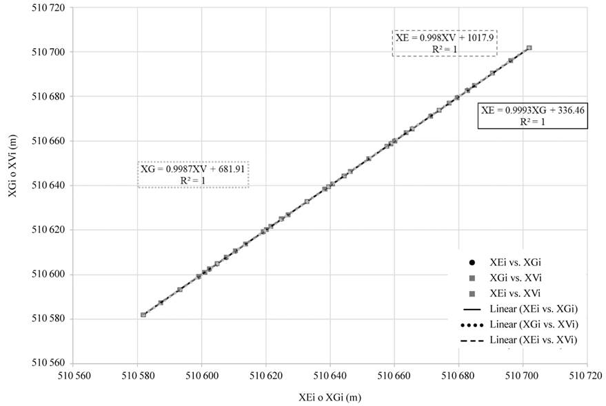
When comparing the variable X of the topographic methods, Figures 3 shows that all three methods have an R2 = 1, a P value of 2.2 x 10⁻¹⁶ for a 95 % confidence level and a residual standard error of 0.022 m between GPS and TS, 0.041 m between TS and UAV, and 0.041 m between GPS and UAV. Therefore, it is considered that there is no significant variation in the length measurements in the three methods.
Y coordinates
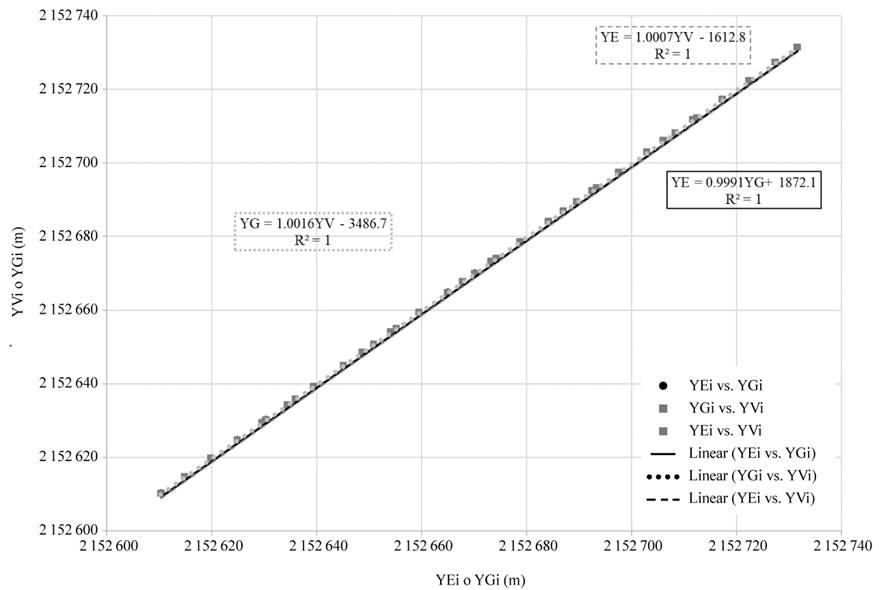
When comparing the Y variable of the survey methods, it is observed that the three techniques have an R2 = 1, a P value of 2.2 x 10⁻¹⁶ for a 95 % confidence level and a residual standard error of 0.018, 0.041 and 0.043 m, for TS vs. GPS RTK, TS vs. UAV and GPS RTK vs. UAV, respectively (Figure 4). Therefore, it is considered that in Y measurements there is no significant difference between the different methods.
Z coordinates
Z coordinate show there is a difference between the different methods. When comparing TS vs. GPS RTK it is observed that R2 is 0.996, with a residual error of 0.010 m and a P value of 2.2 x 10⁻¹⁶ for a confidence level of 95 %, which indicates a concordance of 99 %. On the other hand, when comparing UAV vs. TS it is observed that there is a R2 = 0.743, a residual error of 0.098 m and a P value of 1.44 x 10⁻¹¹ for a 95 % confidence level; likewise, it was obtained a R2 = 0.756, a residual error of 0.092 m and a P value of 5.72 x 10⁻¹² for the same confidence level when comparing UAV vs. GPS RTK.
When analyzing the differences between the variables and for each method, we obtain that when comparing the topographic survey with ST vs. UAV an absolute error of X = 0.061 m, Y = 0.065 m and Z = 0.047 masl is expected, and with GPS RTK vs. UAV an error of X = 0.020 m, Y = 0.002 m and Z = 0.050 masl is expected (Table 3).
Table 3 Statistics of reading differences of variables (X, Y, Z) when comparing three survey methods.
| Variable | TS vs. UAV | TS vs. GPS RTK | GPS RTK vs. UAV | ||||||||
|---|---|---|---|---|---|---|---|---|---|---|---|
| X | Y | Z | X | Y | Z | X | Y | Z | |||
| Maximum | 0.070 | 0.190 | 0.192 | 0.022 | 0.118 | 0.033 | 0.108 | 0.138 | 0.172 | ||
| Minimum | -0.182 | -0.031 | -0.236 | -0.112 | -0.002 | -0.023 | -0.113 | -0.123 | -0.237 | ||
| Average | -0.061 | 0.065 | -0.047 | -0.041 | 0.063 | 0.004 | -0.020 | 0.002 | -0.050 | ||
| Standard deviation | 0.079 | 0.048 | 0.117 | 0.031 | 0.035 | 0.012 | 0.061 | 0.070 | 0.114 | ||
TS = total station; UAV = unmanned aerial vehicle.
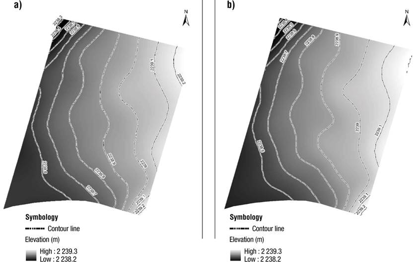
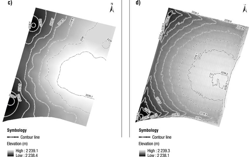
Contour line map
Figures 6 and 7 represent the contour lines generated at 0.1m with the DEMs obtained with each surveying method. The contour lines obtained from TS and GPS RTK surveys are coincidental, and different from those obtained with UAV, which coincides with that reported in Figure 5. It would be pertinent to carry out more tests with UAVs, but with more stable flight devices than those used to achieve a better description of the points on the ground surface, as well as programs with image processing methods that impact on a DEM that better represents reality.
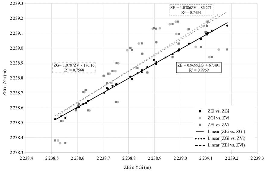
Figure 5 Comparison of Mercator Universal Transverse coordinates (UTM, from zone 14N) altitudinal (Z variables) between the three surveying methods: total station (TS; ZEi), GPS RTK (ZGi) and unmanned aerial vehicle (UAV; ZVi).
Statistical analysis
DEM were compared based on the square root of the root mean square error (RMSE), as analyzed by Komarek, Kumhalova, and Kroulik (2016), and Polat and Uysal (2017). The above is to quantify the magnitude of the deviation of the values obtained in the DEM using UAV in Z variable (elevation), assuming that X and Y variables are coincident according to the DEMs obtained from TS and RTK GPS.
Where z j is the elevation obtained using UAV (m), Z j is the elevation obtained with TS or GPS RTK(m),j = 1, ..., n is the number of each cell (non-dimensional) and n is the number of cells in the raster of the three DEMs.
The estimation of Equation 1 was performed with map algebra of the three DEM rasters (ArcMap [ESRI, 2016]), obtaining the numerator of the function for each cell of the raster estimated. To apply the sum and obtain the number of cells of the raster in the zone spatial analysis tool, the data were exported to a table to sum the values of the squared height differences and obtain the number of cells analyzed (Table 4).
Table 4 Comparison of surveying methods in relation to the square root of the mean square error (RMSE).
| Comparative methods | Number of cells in the raster |
|
RMSE |
|---|---|---|---|
| TS vs. UAV | 3 083 342 | 70 293 | 0.151 |
| GPS RTK vs. UAV | 3 083 342 | 64 573 | 0.145 |
| TS vs. GPS RTK | 3 083 342 | 1 101 | 0.019 |
TS = total station; UAV = unmanned aerial vehicle.
Table 4 shows that RMSE when comparing TS vs. UAV is ±0.151 m, GPS RTK vs. UAV is ±0.145 m, and TS vs. GPS RTK is ±0.019 m.
Gupta and Shukla (2018) report an error of 0.44 between DEM generated with UAV and with TS, which indicates a 65 % difference to the error found in this study. Komarek et al. (2016) obtained an RMSE = 0.29 m when comparing DEM obtained from UAV and GPS RTK, showing a difference of 47 % with respect to the error found in this study. Polat and Uysal (2017) showed an RMSE = 0.171 when generating DEM with UAV and GPS RTK, which agrees with the results obtained in this study, since there is a difference of only 11.7 %.
The MDE obtained from each topographic survey technique does not present significant differences (P ≤ 0.05) in the variables X, Y and Z, which indicates that it is indistinct to use one or another method to generate the MDE with the exposed methodology. When using the equipment analyzed in this study (TS, GPS RTK and photogrammetry), the average error estimated in the variable X is ±0.041 m, and in Y is ±0.043 m. However, in the Z variable the difference is ±0.098 m when compared with X, and with Y it increases by 127 %, so this difference defines the use that will be given to the DEM.
The RMSE statistic of TS vs. UAV is ±0.151 m, of GPS RTK vs. UAV is 0.145 m and of TS vs. GPS RTK is 0.019 m, which indicates that the traditional methods TS and GPS RTK maintain reliability with respect to the photogrammetric method analyzed.
Conclusions
The different surveying methods (ST, GPS RTK and photogrammetry) used to generate a DEM do not differ statistically. According to the conditions described in the study, the user can make a reasoned decision depending on the equipment available and on the application of generating the topography. Furthermore, it was determined that the three methods are reliable, since the traditional methods (TS and GPS RTK) show minor errors compared to photogrammetry using UAV; however, the methods complement each other because it is indispensable to take control points in the field for the georeferencing of DEMs. X and Y coordinates have a lower error, compared to the Z axis in UAVs. For further studies, it is proposed to carry out the survey at different flight heights, and to analyze the error due to the increase in pixel size and surface coverage conditions.

