


 texto em
  Inglês (pdf)
 Artigo em XML
 Referências do artigo
 Enviar este artigo por email
 Citado por SciELO
  Similares em
SciELO
Similares em
SciELO 
 Permalink
Introduction
A topographic survey consists of carrying out a series of activities to measure, calculate and draw the terrestrial surface, as well as determine the position of the points that make up an extension of land (Torres & Villate, 2001). This geo-positioning can be obtained directly or through a calculation process that derives, in the graphical representation of the surveyed terrain, the measurement of the area and volumes of land of interest for civil engineering work (Pachas, 2009). The possibility of obtaining the topography with high spatial and temporal resolution of a site, in the shortest possible time, has been a challenge for various engineering disciplines.
The most commonly used conventional procedures for topographic surveys are based on the use of the global positioning system (GPS), total stations and levels. GPS is capable of capturing information in real time, but the signal may be deficient or suffer distortions when the receiver is located near a building or trees (Fook, 2008). On the other hand, the total station records data of precise discrete points and is used to calibrate new methods, although the resolution or quality of the information depends on the number of points surveyed (Fook, 2008).
Topography has benefited from the emergence of new technologies based on remote sensors mounted on manned and unmanned aerial vehicles (such as satellites, light aircraft or UAVs) that acquire images quickly, which can be processed with photogrammetric techniques in point cloud to obtain digital elevation models (DEMs) (Flener et al., 2013) and orthomosaic (Hernández, 2006). This technology allows obtaining topographic products with greater opportunity; however, it requires specialized programs and Ground Control Points (GCPs) to generate reliable products comparable to those obtained with conventional topographic techniques.
The methodologies derived from high-resolution satellite images such as IKONOS, QuickBird and EROS have been a practical and accessible alternative for the generation of DEMs and topographic information (Fuentes, Bolaños, & Rozo, 2012). This is done through a series of orthorectification and image correction procedures, supported by a set of GCPs that generate terrain elevation models. However, when the images are of low quality (due to cloud cover, atmospheric effects, or shadowing in steeply-sloped or densely-urbanized areas), errors occur in the DEMs (Cavallini, Mancini, & Zanni, 2004).
In recent years, UAVs have become a platform for acquiring digital images and a useful measurement instrument for many surveying applications (Siebert & Teizer, 2014). The main advantage of this equipment lies in the fact that the spatial information captured is denser compared to classical topography works (Hernández, 2006); in addition, it can be applied in coastal zone surveying (Goncalves & Henriques, 2015; Mancini, Dubbini, Gattelli, Stecchi, & Gabbianelli, 2013) and alluvial zone morphological analysis (Tamminga, Hugenholtz, Eaton, & Lapointe, 2014), among other projects.
On the other hand, in most of the work on this topic, the main objective is to obtain a digital surface model (DSM); however, applications in engineering require the digital terrain model (DTM), which excludes constructions and features that protrude from the terrestrial surface (e.g. trees). In this sense, obtaining a DEM with a UAV has the advantage that it allows eliminating the features that are not of interest by editing a point cloud; hence, the end result is a DTM.
Despite the large number of applications using UAVs, the bibliographic information on this subject is still scarce and scattered; in addition, the papers do not always report the accuracy obtained with respect to conventional methods. The topographic products derived from information captured by UAV require validation and local calibration under field conditions to be considered of high accuracy.
Therefore, the objective of this work was to estimate the accuracy of DTMs generated from high-resolution images acquired with a UAV by geolocation of 23 ground points (11 control and 12 verification ones) obtained in the field with a GPS-RTK (Global Positioning System - Real Time Kinematic).
Materials and methods
Study area
The study was conducted in the community of Tlaola, located in the municipality of the same name in the northern highlands of the state of Puebla, Mexico, between geographic coordinates 20° 05’ 18’’ and 20° 14’ 4’’ North latitude, and 97° 50’ 00’’ and 97° 58’ 36’’ West longitude. Aerial images were acquired from 11 a.m. to 2 p.m. on September 1, 2016, and weather conditions were partially cloudy with an average temperature of 17 °C (Weather channel, 2017).
Equipment used
The UAV system used for taking the images was a DroneTools A2 hexacopter. This vehicle performs a vertical takeoff and landing, has a 15-min flight autonomy and a maximum load capacity of 2.5 kg, is equipped with a GPS system that allows running programmed missions and captures images automatically according to the plan flight mission. Additionally, this equipment has a built-in high sensitivity IMU (inertial measurement unit) damper that allows it to have a precise fixed position and altitude, even in wind conditions up to 12 m·s-1 (DJI, 2017).
For this study we used a Sony NEX-7 model α5100 16 mm fixed focal length camera (Figure 1), which captures images with a 24-megapixel sensor (6,000 x 4,000 pixels) in true color. To keep the camera in a positon fixed towards the surface, it was placed on a gyro-stabilized mount.
The terrestrial point coordinates were captured with a TopCon GPS-RTK, which uses two antennas: one works in static mode at a fixed point, with known coordinates, and the other (mobile receiver) is located at each terrestrial point to obtain its coordinates. This equipment provides an accuracy of centimeters (< 1 cm).

Topographic support
Eleven Ground Control Points (GCPs) and 12 Ground Verification Points (GVPs) were located on the ground (Figure 2), obtained with GPS-RTK before the flight for later identification in the images. The GCPs were used to transform the photogrammetric model into a terrain model, while the GVPs were used to quantify the precision of the photogrammetric products obtained.

The GCP and GVP coordinates were obtained with the GPS-RTK on the same day as the flight in the UTM projection system for the 14N zone.
Image acquisition
Three flight missions were carried out to cover a 37.4-ha area in an effective time of 25 min, this considering that the size of the camera sensor is 23.5 x 15.6 mm and the selected flight height was 92 m above the surface, corresponding to a spatial resolution of 2 cm·pixel-1. This height was selected based on two conditions: the first was the optimal spatial resolution to detect the details of the terrestrial surface, and the second was the number of individual images needed to include the entire area, since many individual images make the photogrammetric restitution processes slower (Gómez-Candón, de Castro, & López-Granados, 2014).
On the other hand, images obtained with UAVs must have a high percentage of overlap so that photogrammetric processing can potentially benefit from the resulting redundancy, enabling the generation of high-quality digital models (Haala, Cramer, & Rotherme, 2013). The images should be taken almost parallel to one another and with a frontal and lateral overlap of more than 60 % (Agisoft, 2016), although several authors have had satisfactory results in the generation of digital models with topographic purposes with overlaps greater than 70 % (Eisenbeiss, Lambers, Sauerbier, & Li, 2005; Haala et al., 2013; Lucieer, Jong, & Turner, 2014). Based on these recommendations, the camera was programmed so that images with a lateral and frontal overlap of 75 % were obtained, according to the flight plan shown in Figure 3. With this configuration, 317 images were obtained and then used to generate the DTM from the photogrammetric restitution process.

Generation of digital terrain (DTM) and surface (DSM) models
The program used for the photogrammetric restitution of the images was "PhotoScan" (Agisoft, 2016), in which seven point cloud series were generated using a different number of GCPs (4, 5, 6, 7, 8, 9, 10 and 11), as shown in Figure 4. GCPs were selected taking into account their distribution throughout the study area. The computer used was an HP 8 GB RAM laptop with an Intel Core i7 2.0 GHz processor.
From automatic discretization methods, each point cloud was classified into three classes: terrain, objects and noise. The 'objects' included the points that represent the buildings, trees, vehicles and other elements that are not part of the land; 'terrain' the points that constitute the land, and 'noise' the points with reprojection errors produced in the aerotriangulation process. The latter commonly occur over bodies of water and other moving components, such as vehicles or people in motion.
Finally, the DTMs were generated from the triangulation of the terrain points, and the DSMs, from the triangulation of the terrain and object points.

Accuracy estimation
The evaluation of the accuracy of the DTMs is carried out through the estimation of the statistical errors between the GVP coordinates (in this case 12 points) and those of homologous points considered in the model (Fuentes et al., 2012).
DTMs derived from UAV photogrammetry contain errors, either systematic or accidental, that occur from flight planning to image processing. Systematic errors may be due to the accuracy provided by the GPS with which the coordinates of the GCPs are obtained (Gómez-Candón et al., 2014), the sensitivity of the UAV to the presence of wind (since it is not possible to ensure a regular overlap of the images), the ability of autonomous UAV piloting or the low quality of its sensors (this can randomly affect its altitude and location on the flight) (Nex & Remondino, 2014), the type of UAV selected (multirotor UAVs are more stable than fixed-wing ones) and the geometric accuracy of the camera caused by the distortion of the lens.
On the other hand, accidental errors may be due to the lack of calibration of the camera's internal parameters (Nex & Remondino, 2014), the low percentage (< 70 %) of overlapping between images, the focus of the camera on the flight (since it may not stay fixed, which makes the focal distance vary) (Cabezos & Cisneros, 2012), the number of GCPs selected and their distribution in the field (Grenzdörffer, Engel, & Teichert, 2008), and poor identification of the GCPs in the images within the photogrammetric restitution program (Westoby, Brasington, Glasser, Hambrey, & Reynolds, 2012).
The accuracy of the DTMs was evaluated with the total errors, which involve the errors present from the planning of the flight until the generation of the models with the photogrammetric technique, for which four statistical error parameters were calculated (Equations 1 to 4): the mean error (ME), the root-mean-square error (RMSE), the standard deviation of the error (SDE) and the maximum absolute error (Emax). ME is a measure of the accuracy of the data that indicates any positive or negative systematic error, RMSE is a dispersion measure of the frequency distribution of the residuals that is sensitive to large errors, SDE provides information on the accuracy and distribution of the residuals around the average and Emax describes the greater residual present for understanding the quality limits of the data (Willmott & Matsuura, 2005). The residuals (Ccal-Cobs) on each axis were calculated as the difference between the measurements taken from the DTMs and those taken with the GPS-RTK on the plane (X, Y, Z) (Equation 5). Positive values indicate overestimation of data from the DTM, and negative values indicate underestimation of data by the DTM.
Where: Ccal = coordinates x, y, z extracted from the DTM in the GVPs and Cobs = coordinates of the GVPs measured with the GPS-RTK.
The SDE for each axis should not be understood as the maximum error of the DTM on that axis, but as an indicator of the overall error. Assuming a normal distribution of errors, 68.27 % of the errors are below the indicated SDE, 95.45 % twofold below the SDE and 99.76 % threefold below the SDE.
Results and discussion
Generation of DTM and DSM
For each of the seven photogrammetric restitutions, a dense cloud of points, a DSM, a DTM and an orthomosaic were obtained; the main characteristics of these photogrammetric products are shown in Table 1.
Table 1 Characteristics of the photogrammetric products obtained.
| Characteristic | Value |
|---|---|
| Surface (ha) | 37.4 |
| No. of processed images | 317 |
| Total | 64,820,000 |
| Points in the dense cloud Of terrain | 27,702,639 |
| Points in the dense cloud Of objects | 37,114,821 |
| Noise | 2,540 |
| Resolution of the DSMs and DTMs* | 8.39 cm·pixel-1 (142 points·m-2) |
| Resolution of the orthomosaic | 2 cm·pixel-1 |
*DSMs: digital surface models; DTM: digital terrain models.
The photogrammetric workflow, which included the field and office stages, was carried out at 21.5 h (Figure 5). The image processing stage for the generation of the DTMs demanded 72.6 % of the time required (equivalent to 15.6 h), the surveying of the GCPs and GVPs required 14.0 %, image acquisition (flight times, UAV assembly, battery change and transfer to takeoff points) demanded 11.2 % and the programming of the flight missions 2.3 %. The times that were required to travel to the study site are not considered. Nex and Remondino (2014) mention that the image processing stage requires the most time in photogrammetric work with UAV, approximately 60 %; although in this work it was greater, it can be improved if a computer with a greater processing capacity is used.
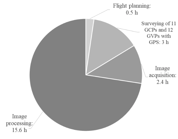
Figure 5 Times used in the photogrammetric workflow with a unmanned aerial vehicle (UAV) for 37.4 ha.
Within the image processing stage, the discretization of the dense point cloud into three classes was a fundamental step to obtain the models representing the study site’s topography. The discretization allowed triangulating only the terrain points to generate the DTMs, in addition to separating the noise points to avoid undesired effects in the creation of the mesh (Peinado-Checa, Fernández, & Agustín-Hernández, 2014). Noise points were found mainly on the surface of the Ixtacatla River, which crosses the town of Tlaola. Figure 6 shows the discretization of a point cloud in the terrain, objects and noise classes, where it can be seen that the class with the highest number of points was objects (57.258 %), since the flight was made over an urban area, followed by terrain (42.738 %) and noise (0.004%).

The DSMs (Figure 7) of high spatial resolution represent in great detail the characteristics of the surface, such as the surface roughness, the vegetation that makes up the landscape, and buildings, among others. On the other hand, the DTMs (Figure 8) only show characteristics of the surface terrain without considering the protruding objects. This last case is of special interest in engineering, since it can be used to generate contours and longitudinal and cross-sectional profiles.


The DTMs provide a density of 142 points·m-2, which allows detecting small terrain details. This density was a function of the resolution at which the images were acquired and the quality (very low, low, medium, high and very high) of the processing in "PhotoScan". Generally, this type of technology can provide a density greater than 100 points·m-2 (Cryderman, Bill-Mah, & Shufletoski, 2015; Neitzel & Klonowski, 2012) in a relatively short time, which could not be achieved with conventional technologies such as total station or GPS.
Accuracy estimation
The ME of the DTM generated with four GCPs was less than 11 cm on the X and Y axes, while on Z it was greater than 2 m. This DTM greatly overestimated terrain elevations, indicating that the number of GCPs used for its georeferencing are not sufficient; however, the errors in X and Y are not so large because the percentage of overlap between images had a greater influence than the number of GCPs. For the rest of the DTMs, the ME values on the three axes were less than 2 cm, which shows that the number of points and their distribution are important in determining the accuracy of the models, since GCPs were used in the corners and near the center of the study area.
In the analyses with the RMSE, it was found that the DTMs have a greater error on vertical (Z) than horizontal (X and Y) axes. The DTM with four GCPs has a value greater than 3 m on the Z axis, and with five or more GCPs have errors of less than 5, 4 and 12 cm on the X, Y and Z axes, respectively. This again highlights the importance of having GCPs in the central area of the study area. The RMSE, in comparison with the ME, amplifies and penalizes with greater force those errors of greater magnitude.
In these digital models, as errors are greater in the vertical than in the horizontal, several authors have quantified the error only on the vertical axis with the support of a multirotor UAV, finding an RMSE of 8.8 cm (Tamminga et al., 2014) and 6.6. cm (Uysal, Toprak, & Polat, 2015), while Hugenholtz et al. (2013), when using a fixed-wing UAV, obtained an RMSE of 29 cm. This shows that the accuracy on the three axes of the digital models generated by photogrammetry using UAV can be less than 10 cm. Nex and Remondino (2014) mention that the RMSE of these models is generally two to three times the pixel size of the acquired images (or the spatial resolution of the orthomosaic). In this case, the georeferenced models with 9, 10 and 11 GCPs have an RMSE of less than 10 cm in the three axes; however, only the model georeferenced with 11 GCPs has an RMSE (5.9 cm) of less than three times the resolution of the orthomosaic (2 cm·pixel-1). Therefore, the latter could represent the site’s topography with high accuracy.
Because the DTM referenced with 11 GCPs is the one with the best accuracy and the one that best represents the site’s topography, according to the SDE, the accuracy on the Z axis was less than 5.8 cm in 25.53 ha (68.27 % of the total surface), 11.6 cm in 35.70 ha (95.45 %) and 17 cm in 37.31 ha.
The Emax, like the other estimators, was greater on the Z axis. The Emax that was found in all the DTMs on the plane (X, Y, Z) was in GVP 10, because it is located in an area (near the edge) with less than six overlapping images, while the other points present at least nine images for photogrammetric restitution. In photogrammetric surveys near the edge of the surveyed area, the number of overlapping images is smaller with respect to the central area; therefore, it is advisable to program the flight mission for a larger area of the area of interest, in such a way that a minimum number of overlapping images (nine) images is ensured. On the other hand, one should avoid locating terrestrial points near the boundaries of the area of interest.
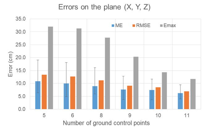
Table 2 shows the comparison of the errors calculated for the DTMs generated from different CP numbers. The statistical errors of the digital models on the plane (X, Y, Z) (Figure 9) decreased when the number of GCPs used for their georeferencing increased. The accuracy of digital models on X and Y remains stable (RMSE < 5 cm) from five GCPs, while on the Z axis a greater influence of the number of points is observed, since the values of the RMSE were found to be greater than 10 cm when less than nine points were used.
Table 2 Comparison of statistical errors between digital terrain models and GPS-RTK measurements.
| Eje | Parameters (cm) | Number of ground control points | ||||||
|---|---|---|---|---|---|---|---|---|
| 4 | 5 | 6 | 8 | 9 | 10 | 11 | ||
| X | ME* | 6.5 | -0.4 | 1.7 | 0.5 | 0.0 | -0.1 | 0.3 |
| RMSE | 9.4 | 4.3 | 5.2 | 3.0 | 3.7 | 3.7 | 2.1 | |
| SDE | 7.1 | 4.5 | 5.1 | 3.0 | 3.8 | 3.8 | 2.2 | |
| Emax | 16.2 | 9.4 | 10.9 | 5.3 | 7.4 | 10.2 | 4.1 | |
| Y | ME | 10.5 | 0.0 | 0.9 | 0.6 | -0.1 | 0.0 | 1.3 |
| RMSE | 11.6 | 3.2 | 3.0 | 2.7 | 3.3 | 3.8 | 3.0 | |
| SDE | 6.8 | 3.4 | 3.0 | 2.7 | 3.4 | 3.9 | 2.8 | |
| Emax | 17.8 | 6.0 | 6.4 | 5.8 | 6.2 | 7.4 | 6.9 | |
| Z | ME | 275.5 | 0.0 | 1.5 | 1.2 | 0.3 | -0.6 | 2.1 |
| RMSE | 304.1 | 12.2 | 11.2 | 10.5 | 7.7 | 6.6 | 5.9 | |
| SDE | 134.5 | 12.8 | 11.6 | 10.9 | 8.0 | 6.9 | 5.8 | |
| Emax | 400.7 | 30.0 | 29.0 | 27.0 | 18.0 | 12.2 | 10.9 | |
| Average (X, Y, Z) | ME | 276.0 | 10.9 | 10.0 | 9.0 | 7.6 | 7.5 | 6.2 |
| RMSE | 304.5 | 13.4 | 12.7 | 11.2 | 9.1 | 8.5 | 7.0 | |
| SDE | 134.2 | 8.2 | 8.1 | 7.1 | 5.2 | 4.2 | 3.2 | |
| Emax | 401.2 | 32.0 | 31.3 | 27.7 | 20.3 | 14.4 | 11.7 | |
*ME: mean error; RMSE: root-mean-square error; SDE: standard deviation of the error; Emax: maximum absolute error.
*ME: mean error; RMSE: root-mean-square error; Emax: maximum absolute error.
Figure 9 Statistical errors of the digital terrain models on the plane (X, Y, Z).
The results show that accuracy of less than 10 cm (in the three axes) can be obtained in the DTMs derived from photogrammetry with UAV. This accuracy is greater than that obtained with other remote sensing technologies, as is the case of Fuentes et al. (2012), who used IKONOS satellite images and found accuracies of 1.49, 3.5 and 3.89 m on the X, Y and Z axes, respectively. On the other hand, Zhang, Pateraki, and Baltsavias (2002) obtained five DEMs with five different interpolation algorithms using IKONOS images and found RMSE values on the Z axis from 3.1 m to 5.4 m. With airborne LiDAR sensors, Bowen and Waltermire (2002) report an RMSE in the vertical of 43 cm, Legleiter (2012) of 21 cm and Notebaert, Verstraeten, Govers, and Poesen (2009) of 15 cm in the Belgian river valleys. However, there are other technologies such as terrestrial laser scanners that can provide accuracies of the order of 4 cm on Z (Williams et al., 2013), although with a cost of resources and time greater than with the use of UAVs.
Conclusions
Information capture by UAVs allows generating a greater number of points, which improves the level of detail with which the surface is represented in the models. The DTMs generated have a spatial resolution of 8.4 cm·pixel-1, equivalent to 142 points·m-2, and provide a level of detail that is not possible to obtain with traditional topographic equipment.
The most reliable statistical parameter to determine the accuracy of the models is the RMSE since it is sensitive to large errors. In turn, the ME estimator provides useful information, but it is not recommended when large-magnitude errors occur.
The largest errors in the DTMs were found on the Z axis. The number of GCPs in the terrain had a considerable impact on the accuracy of the DTMs, especially on the Z axis; that is, if the number of GCPs is low, accuracy is guaranteed on X and Y, but not on Z. The RMSEs on X and Y of the DTMs georeferenced with more than five GCPs were less than 5 cm, which shows little influence of the number of GCPs on the accuracy on these axes, while on Z they were greater than 10 cm when less than nine points were used.
The DTM georeferenced with 11 GCPs represented the site’s topography with better accuracy, since the highest RMSE, which was presented on the Z axis, was 5.9 cm, which is three times less than the spatial resolution of the orthomosaic (2 cm·pixel-1). Therefore, at least five terrestrial GCPs well-distributed throughout the study area are essential for every 15 ha of surveyed surface; in addition, it is necessary to add one point for each additional 3 ha to obtain a minimum accuracy (RMSE) of 6 cm on the Z axis and 7 cm on the plane (X, Y, Z).
Additionally, the frontal and lateral overlap of the images play an important role, since they determine the number of images in which the same point is observed. A minimum average frontal and lateral overlap of 75 % ensures an adequate number of points in the DTM. In addition, the flight mission must be programmed for a larger area of the area of interest, since near the limits of the flight area where few images overlap, the accuracy is less than in the central areas.
Finally, we were able to determine that the digital models derived from UAV photogrammetry are of high spatial resolution and can provide accuracies of less than 10 cm on the three axes. Therefore, this technology can be adopted in the field of topography, since these models are also obtained in shorter times and with fewer resources than conventional technologies such as total stations and differential GPS. However, both technologies should be considered complementary, because it is essential to obtain terrestrial GCPs for the georeferencing of digital models.

