


 texto em
  Inglês (pdf)
 Artigo em XML
 Referências do artigo
 Enviar este artigo por email
 Citado por SciELO
  Similares em
SciELO
Similares em
SciELO 
 Permalink
Highlights:
Topographic conditions influence the vertical and spatial structure of Lippia graveolens.
Basal diameter and height were higher on slopes than on plains and ravines.
The number of branches and basal area were higher on the southeast exposure and on steep slopes
The spatial distribution of oregano is clustered and sometimes random.
Introduction
Oregano (Lippia graveolens H. B. K.) is an aromatic plant used as a condiment and for medicinal use (García-Pérez, Castro-Álvarez, Gutiérrez-Uribe, & García-Lara, 2012). Oregano oil is used in the production of soaps, perfume, cosmetics and flavorings (Koksal, Gunes, Orkan, & Ozden, 2010). This species grows in 24 states of Mexico under climates with precipitation between 300 and 400 mm per year (Soto, González, & Sánchez, 2007). Oregano has threatened wild populations, due to overgrazing and overharvesting of plants for commercialization (Osorno-Sánchez, Flores-Jaramillo, Hernández-Sandoval, & Lindig-Cisneros, 2009; Osorno-Sánchez, Torres, & Lindig-Cisneros, 2012).
The structure of a population is the result of the action of biotic agents such as dispersers, predators and competitors; abiotic agents such as climate, soil, relief and geology to which members are subject (Letcher et al., 2012); and human-induced disturbances such as vegetation use and grazing (Ayerde-Lozada & López-Mata, 2006).
The structure of a population can be characterized with the vertical ordering of strata per height category, and horizontal ordering with the use of spatial distribution indices (Zarco-Espinosa, Valdez-Hernández, Ángeles-Pérez, & Castillo-Acosta, 2010). The spatial distribution pattern of a species is useful for understanding ecological processes such as competition, symbiosis, and dispersal (Law et al., 2009). The distance between individuals can reflect processes of seed dispersal, competition and predation, along with the result of environmental constraints, which will define the spatial structure of the population (Gómez, 2008).
Information on the current status of L. graveolens populations in the Tehuacán Cuicatlán Biosphere Reserve is scarce. In this context, the objective of the present study was to determine the vertical structure and spatial distribution of L. graveolens under different topographic conditions. The hypothesis proposes that the vertical structure and spatial distribution are different between topographic conditions, because exposure and slope modify the microclimatic context as found in the species Carnegiea gigantea (Engelm.) Britton & Rose and Neobuxbaumia tetetzo (F. A. C. Weber ex K. Schum.) Backeb (López-Gómez, Zedillo-Avelleyra, Anaya-Hong, González-Lozada, & Cano-Santana, 2012).
Materials and Methods
Study area and sampling
The study was carried out in the ejido Santa María Coapan, Tehuacán, Puebla, located at the Tehuacán-Cuicatlán Biosphere Reserve (RBTC), between the geographical coordinates 18° 23´ 26.85´´ - 18° 23´ 0.31´´ N and 97° 23´14.93´´- 97° 22´17.53´´ W (Figure 1), at an average altitude of 1 465 m.
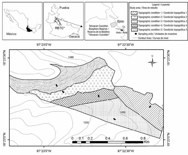
Figure 1 Location of the study area of Lippia graveolens, topographic conditions and sampling units at the Tehuacán-Cuicatlán Biosphere Reserve (RBTC), Mexico.
Five topographic conditions were identified based on topoform, exposure and slope of the soil (Figure 1; Table 1). Exposure was obtained with the 1:50 000 scale digital elevation model (Instituto Nacional de Estadística y Geografía [INEGI], 2013), using "aspect" from ArcGis V.10.5 software (Environmental Systems Research Institute [ESRI], 2016) as a geoprocessing tool. Slope was measured with a Suunto clinometer. Oregano plant variables were measured under a targeted systematic sampling design, where two contiguous 250 m2 (10 x 25 m) sampling units were located at each topographic condition.
Table 1 Characterization of five topographic conditions (TC) of Lippia graveolens populations at the Tehuacán-Cuicatlán Biosphere Reserve, Mexico.
| Topographic conditions | Topoform | Exposure | Slope (%) |
|---|---|---|---|
| TC1 | Plain | Zenith | 0 |
| TC2 | Ravine | East | 15 |
| TC3 | Hillslope | East | 8 |
| TC4 | Hillslope | North | 31 |
| TC5 | Hillslope | Southeast | 65 |
Population structure
L. graveolens plants were enumerated and located on the Cartesian plane (X, Y) of the sampling units. Height (cm), basal diameter (mm) of each stem and number of stems of each plant were recorded in September 2019. The number of plants counted in the sampling units was extrapolated to estimate plant density∙ha-1. Six plant height categories of L. graveolens were defined based on the sampling carried out: 1 = 0 to 50 cm, 2 = 51 to 100 cm, 3 = 101 to 150 cm, 4 = 151 to 200 cm, 5 = 201 to 250 cm and 6 = >251 cm. For each topographic condition, population structure curves were constructed with the percentage of plants in the height categories and compared to each other with the Ӽ2 test. Moreover, curves were classified according to typical structural types (Bongers, Popma, Meave-del Castillo, & Carabias, 1988; Martínez-Ramos, & Álvarez-Builla, 1995; Peters, 1994; Velasco-García, Valdez-Hernández, Ramírez-Herrera, & Hernández-Hernández, 2017): type I (Bongers = Peters' type I) has high frequency of individuals in the first or second diameter class and gradual decrease in higher classes; type II (Bongers = Peters' type II = Martínez-Ramos' type III) has high frequency of individuals in the first diameter class, second or third class poorly represented, increased frequency in intermediate classes, and decrease in higher classes; type IIb (Velasco-García) has low proportion of the first category, decrease in the next two categories, increase and high proportion of intermediate categories and drastic decrease in the rest of the higher categories; type III (Bongers = type I of Martínez-Ramos) has 50 % or more individuals in the first diameter class and very low and uniform frequency in the following classes; type IV (Velasco-García) with low frequency in the first category, high frequency in the second category, very low frequency in the third and fourth categories, high frequency in the fifth category and low frequency with gradual decrease in the rest of the categories.
The importance value index (IVI = relative density + relative dominance + relative frequency) (Ajayi & Obi, 2016) was calculated treating height categories as distinct elements in each topographic condition (Velasco-García et al., 2016).
The assumption of normality of structural attributes was examined with the Shapiro-Wilks test. Height and importance value index met the assumption of normality; therefore, analysis of variance (ANOVA) and Tukey's mean comparisons (P ≤ 0.05) were performed. Basal diameter, number of stems and basal area did not meet the assumption of normality, so nonparametric tests of variance and Kruskal-Wallis multiple comparisons (P ≤ 0.05) were performed. All analyses were carried out using the statistical program InfoStat version 2019 (Di Rienzo et al., 2019), with the model Yij = µ + Ci + εij; where, Y ij is the observation value, μ is the effect of the overall mean, C i is effect of the i-th topographic condition and ɛ ij is the effect of the experimental error.
Spatial distribution pattern
For the analysis of spatial distribution, the two contiguous sampling units in each topographic condition were used as a single sampling unit (20 x 25 m = 500 m2). Perpendicular distances between the sampling unit boundaries (width and length) and between each of the plants were measured to locate them on a Cartesian plane. The spatial distribution pattern of L. graveolens plants was determined with the Ripley's transformed function (K
(t)
):
Results and Discussion
Population structure
Based on Table 2, the structural attributes of L. graveolens showed significant differences (P < 0.05) among topographic conditions (TC). TC3 had the plants with the highest height and basal diameter, and TC5 also had the plants with the highest height. In contrast, TC2 and TC1 had the lowest values for both variables. The average plant height was 32 % higher in TC5 compared to TC2 and the basal diameter was 21 % higher in TC3 compared to TC2.
Table 2 Structural attributes of Lippia graveolens under five topographic conditions at the Tehuacán-Cuicatlán Biosphere Reserve, Mexico.
| Topographic conditions | Height (cm) | Basal diameter (mm) | Number of stems | Basal area (cm2) |
|---|---|---|---|---|
| TC1 | 136.8 bc | 10.4 c | 3.2 c | 4.0 c |
| TC2 | 125.3 c | 10.0 c | 3.6 bc | 3.9 c |
| TC3 | 165.1 a | 12.1 a | 3.5 b | 5.4 ab |
| TC4 | 151.4 ab | 11.6 ab | 3.4 bc | 4.9 b |
| TC5 | 165.6 a | 11.9 b | 4.3 a | 7.3 a |
| Mean | 148.8 | 11.2 | 3.5 | 5 |
Mean values of height with different letters are significantly different according to the Tukey's test (P < 0.05). Mean values of basal diameter, number of stems and basal area with different letters are significantly different among topographic conditions according to the Kruskal-Wallis test (P < 0.05). TC features are shown in Table 1.
Topoform, exposure and slope may be the cause of differences in height and basal diameter of L. graveolens. In general, plain and gully topoforms had plants with lower plant diameter and height compared to hillslopes. It has been reported that arid ecosystem sites with northern exposure have higher moisture and lower temperature and evapotranspiration, which favors plant growth (Bochet, García-Fayos, & Poesen, 2009). Moreover, Carrasco-Ríos (2009) and Raffo (2014) indicate that plants develop better in the southern and eastern exposures, because they receive more solar radiation compared to the northern exposure slopes. In agreement with the aforementioned, although TC3 and TC2 had the same exposure (east), TC3 had plants with higher height and basal diameter, due to the lower slope (8 %) of the terrain. On the other hand, TC4, despite the high slope (31 %), also had higher plant height due to its location on the northern exposure. In contrast, topographic condition 5, even though it was located on the southeast exposure and on a steeper slope, had taller plants, possibly because most of them were adults. Oregano generally grows in very shallow soils with low amounts of organic matter and steep slopes (González, 2012; Granados-Sánchez, Martínez-Salvador, López-Ríos, Borja-De la Rosa, & Rodríguez-Yam, 2013); however, besides exposure and slope, there are other environmental factors such as climate, water, and geology that can affect plant growth (Niua et al., 2014).
In the present study, the average height of L. graveolens (148.8 cm) was higher than in semidesert plants in Querétaro (69.9 cm; Osorno-Sánchez et al., 2012) and the Comarca Lagunera (94.8 cm; Flores et al., 2011). This difference may be due to the level of disturbance in these regions. In the wild populations of Querétaro, Coahuila, Durango, and Chihuahua, L. graveolens plants are cut at early ages to sell the foliage as a condiment in the local and national market (Granados-Sánchez et al., 2013; Orona, Salvador, Espinoza, & Vázquez, 2017). Taller plants can have a high foliage quantity, so these are cut and smaller plants are left behind. This causes changes in plant size structures in populations where this species is collected (Flores et al., 2011; Osorno-Sánchez et al., 2012). Also, livestock grazing can influence plant size due to browsing. In contrast, disturbance from harvesting and grazing is minimal for L. graveolens populations in the RBTC, which causes plants to reach the maximum growth allowed by the environment. The populations of this species in the reserve are not subject to harvesting based on a management program, as is the case with populations in northern Mexico. Furthermore, the environmental conditions are different in the state of Puebla, compared to those of other states where L. graveolens grows; for example, annual precipitation is 437 mm and mean annual temperature is 20.5 °C in the RBTC (Rehfeldt, 2006), while in ecosystems of the states of Guanajuato, Querétaro, Coahuila, Durango and Chihuahua, mean annual precipitation is reported between 125 to 400 mm and mean annual temperatures between 15 to 21 °C (Granados-Sánchez, Sánchez-González, Granados, & Borja, 2011; Ocampo-Velázquez, Malda-Barrera, & Suárez-Ramos, 2009).
TC5 had significant differences (P ≤ 0.05) compared to the other conditions in the number of stems and basal area, which were 34 % and 87 % higher, respectively, than the values of TC1, TC2 and TC4. This occurred possibly because the slope is steeper and the exposure is southeast in TC5; in addition, it has more open space. The above suggests that steep slopes and southeast exposure positively influence the number of oregano stems and basal area.
The orientation of the slopes modifies the microclimatic conditions and influences the architecture of the plant; for example, N. tetetzo had a higher number of branches in the northern exposure (López-Gómez et al., 2012). As a result, wind can cause damage to the main stem of oregano seedlings, promoting a higher number of stems and, consequently, a larger basal area. In addition, plants may emit a higher number of stems when grown in populations with lower densities (Salomón-Montijo, Reyes-Olivas, & Sánchez-Soto, 2016).
The average number of stems (3.5) of oregano in this study was lower than in oregano populations in Coahuila and Durango (8.7; Flores et al., 2011). This may be a consequence of use of foliage in those states (Orona et al., 2017), where pruning promotes shoot emergence (Granados-Sánchez et al., 2013; Osorno-Sánchez et al., 2009). Based on the above, use of foliage in L. graveolens plants can generate a higher number of stems.
According to Table 3, density ranged between 1 820 and 6 240 plants∙ha-1 in TC2 and TC1, respectively. Density, without considering topographic conditions, was higher (4 044 plants∙ha-1) than densities in oregano populations in Querétaro (3 891 and 2 450 plants∙ha-1; Osorno-Sánchez et al., 2009, 2012) and in Tamaulipas (905 plants∙ha-1; Sánchez-Ramos, Quezada, Lara-Villalón, Medina-Martínez, & Pérez-Quilantán, 2011). Differences may be due to the lack of harvesting and low disturbance in the study population, because there is no management program and people do not illegally harvest the species, because as the extraction of L. graveolens plants increases, density decreases as a consequence of altered mortality and selection rates (Osorno-Sánchez et al., 2009, 2012). Also, the slope may influence plant density due to the dragging of seeds from the upper parts (steep slopes) to areas with lower slope, which allows a higher plant abundance in these areas (Grasty, Thompson, Hendrickson, Pheil, & Cruzan, 2020).
Table 3 Density of Lippia graveolens in five topographic conditions (TC) per altitude categories at the Tehuacán-Cuicatlán Biosphere Reserve, Mexico.
| Height category | Density (plants∙ha-1) | ||||
|---|---|---|---|---|---|
| TC1 | TC2 | TC3 | TC4 | TC5 | |
| 1 (1-50 cm) | 760 | 120 | 40 | 80 | 20 |
| 2 (51-100 cm) | 1 340 | 460 | 380 | 460 | 300 |
| 3 (101-150 cm) | 1 080 | 680 | 1 000 | 1 700 | 800 |
| 4 (151-200 cm) | 1 840 | 480 | 2 320 | 2 200 | 980 |
| 5 (201-250 cm) | 1 120 | 40 | 720 | 340 | 660 |
| 6 (>251 cm) | 100 | 40 | 60 | 20 | 80 |
| Total | 6 240 | 1 820 | 4 520 | 4 800 | 2 840 |
The description of TC is shown in Table 1.
The highest number of oregano plants was recorded in height category 4 (201-250 cm) in all topographic conditions except for TC2. The lowest plant density was found in category 1 (1-50 cm) of TC5 and in category 6 (>251 cm) of TC4 (Table 3). TC1 had the highest number of plants in category 1 compared to the other topographic conditions for this category. The presence of a higher number of small plants in TC1 may be due to the flat terrain, which contains a higher concentration of nutrients in the soil than the higher parts, favoring the regeneration of oregano plants (López-Acevedo et al., 2004). The results showed a low number of plants in the lower and higher height categories. This may reflect that new oregano plants are selected only in years with favorable environmental conditions (Osorno-Sánchez et al., 2012).
Population structures of L. graveolens were different (P < 0.05) among the five topographic conditions. Type IV curve (Velasco-García et al., 2017) was found in TC1 (Figure 2). This curve type had a low percentage of plants (<20 %) in height categories 1, 3, 5 and 6, and slightly higher (20 to 30 %) in categories 2 and 4. The above may be due to biotic and abiotic constraints for fruit and seed production (Velasco-García et al., 2017), so there is discontinuous selection in larger height categories. Fruit production of L. graveolens depends on pollinators of the genus Melipona (Ocampo-Velázquez et al., 2009); the temporary absence of these can disrupt seed regeneration (Ocampo-Velázquez et al., 2009); moreover, fruit production of L. graveolens only occurs in 11.4 % of the total flowers (Ocampo-Velázquez et al., 2009).
TC2 to TC5 had population structure different from typical population structure curves (Bongers et al., 1995; Martínez-Ramos & Álvarez-Builla, 1995; Peters, 1994; Velasco-García et al., 2017), which was called V-type curve (Figure 2). This type of curve was characterized by a very low percentage in height category 1, gradual increase in the following categories up to high percentage in the intermediate category and gradual decrease in higher categories up to very low percentage in the last category. A similar population structure curve was reported for populations of Dioon holmgrenii De Luca, Sabato & Vazquez Torres disturbed by grazing (Velasco-García et al., 2016). The V-type population structure in L. graveolens may be due to factors limiting regeneration such as low seed germination percentage, due to extreme environmental conditions (temperature and moisture) in arid areas that may influence selection of new individuals (Martínez, Blando, Morales, & Gómez, 2013; Martínez-Hernández, Villa-Castorena, Catalán-Valencia, & Inzunza-Ibarra, 2017). Increasing harvest rate causes changes in the population structure curve of L. graveolens, from type I curve (Bongers et al., 1988) in areas with low harvest, going through type II curve (Martínez-Ramos & Álvarez-Builla, 1995), to type V curve in areas with high harvest rate (Osorno-Sánchez et al., 2009, 2012). In the present study, despite the absence of oregano harvesting and differences in exposure and slope, the type V population structure curve seems to be common in this species; however, the flat soil and zenithal exposure did not favor oregano selection, which generated the type IV curve.
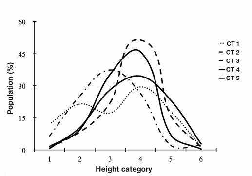
Figure 2 Population structure curves per height categories (1 = 1-50 cm, 2 = 51-100 cm, 3 = 101-150 cm, 4 = 151-200, 5 = 201-250 cm, 6 > 251 cm) of Lippia graveolens in the five topographic conditions (TC) at the Tehuacán-Cuicatlán Biosphere Reserve, Mexico.
IVI was different (P < 0.05) among height categories in each of the topographic conditions. According to Table 4, the highest IVI was found in height category 4 (151-200 cm) in all TC, while height category 1 (seedling) had low values. These results are consistent with the average density of the height categories and population structure curves, which also showed the null extraction of reproductive oregano plants in this zone; however, natural regeneration is deficient, due to multiple biotic and abiotic factors that require more detailed studies.
Table 4 Importance value index (IVI) per height category of Lippia graveolens in five topographic conditions (TC) at the Tehuacán-Cuicatlán Biosphere Reserve, Mexico.
| Height categories | Importance value index | ||||
|---|---|---|---|---|---|
| TC1 | TC2 | TC3 | TC4 | TC5 | |
| 1 (1-50 cm) | 27.4 b | 12.7 b | 9.7 c | 11.5 b | 8.9 c |
| 2 (51-100 cm) | 40.5 b | 56.1 ab | 31.7 bc | 33.2 b | 31.6 bc |
| 3 (101-150 cm) | 42.3 b | 100.7 ab | 53.4 bc | 85.8 a | 60.3 ab |
| 4 (151-200 cm) | 92.8 a | 103.7 a | 126.1 a | 118.2 a | 95.9 a |
| 5 (201-250 cm) | 71.4 ab | 15.3 ab | 65.7 b | 40.0 b | 73.5 ab |
| 6 (>251 cm) | 25.6 b | 11.5 b | 13.5 c | 11.3 b | 29.8 bc |
| Total | 300 | 300 | 300 | 300 | 300 |
Mean values of IVI with different letters are significantly different between height categories according to Tukey's test (P < 0.05) for each TC. Description of the TC is shown in Table 1.
Spatial distribution
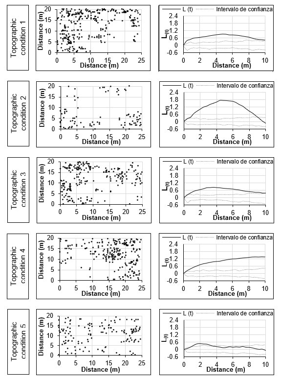
Figure 3 indicates that the distribution pattern of L. graveolens plants was aggregated (P ≤ 0.01) for TC1 to TC4. Maximum clustering occurred at t distances of 4.8 m (L (t) = 0.93) in TC1, 4.4 m (L (t) = 1.74) in TC2, at 3.6 m (L (t) = 0.84) in TC3, and at 8.8 m (L (t) = 1.35) in TC4. The spatial distribution of plants was both random and aggregated for TC5 (P ≤ 0.01). The aggregated spatial distribution of L. graveolens is influenced by the slope; TC1 to TC4 had lower percentages of slope compared to TC5 (65 %). The aggregate distribution pattern of plants may be associated with topography (Linzaga-Román, Ángeles-Pérez, Catalán-Heverástico, & Hernández-De la Rosa, 2011) and may indicate interactions among individuals and between individuals with the environment (Linzaga-Román et al., 2011; Ruiz-Aquino, Valdez-Hernández, Romero-Manzanares, Manzano-Méndez, & Fuentes-López, 2015). Limitations in terms of seed dispersal distance can lead to an aggregate distribution pattern (Lara-Romero, de la Cruz, Escribano-Ávila, García-Fernández, & Iriondo, 2016) around the mother plant. This occurs in L. graveolens, when the fruits ripen, the seeds are expelled and fall to the ground near the plant (Martínez et al., 2013, 2017).
The random spatial distribution in TC5 (Figure 3) is due to the steeper slope that may influence the distribution and germination of seeds in the soil, which are commonly dispersed by the wind (Martínez et al., 2013). Mortality of seeds or seedlings of some species is likely to cause greater distances between survivors, reflecting a less clumped pattern (Vallejo & Galeano, 2009). Random spatial distribution contributes to multifunctionality related to nutrient cycling in a plant community (Maestre, Castillo-Monroy, Bowker, & Ochoa-Hueso, 2012).
Conclusions
Soil topographic conditions influenced the vertical structure and spatial distribution of Lippia graveolens. The slope condition positively influenced plant diameter and height. Southeast exposure and steep slopes positively affected branch number and basal area. Also, a low number of new shoots and few senescent individuals were found, indicating little regeneration and that the population may decrease. The type V population structure curve (low frequency in the first category, gradual increase up to the intermediate category and gradual decrease in the rest) was common; however, the flat condition and zenithal exposure were not favorable for the selection of L. graveolens, generating the type IV curve (low frequency in the first, third and fourth height categories, high in the second and fifth, and low in the rest). The spatial distribution of oregano was commonly clustered, but the high slope of the ground also caused the random distribution.

