


Serviços Personalizados
Journal
Artigo
 texto em
  Inglês (pdf)
 Artigo em XML
 Referências do artigo
 Enviar este artigo por email
Indicadores
-
 Citado por SciELO
 -
 Acessos
Links relacionados
-
 Similares em
SciELO
Similares em
SciELO
Compartilhar

 Permalink
Tecnología y ciencias del agua
versão On-line ISSN 2007-2422
Tecnol. cienc. agua vol.10 no.3 Jiutepec Mai./Jun. 2019 Epub 21-Abr-2021
https://doi.org/10.24850/j-tyca-2019-03-04
Articles
Physical modeling of erosion in low height structures with ski jumps
1
 http://orcid.org/0000-0003-0624-5781
3
http://orcid.org/0000-0002-5594-4848
1Universidad Nacional de Córdoba, Córdoba, Argentina; Consejo Nacional de Investigaciones Científicas y Técnicas (Conicet), Buenos Aires, Argentina, matiaseder@unc.edu.ar
2Universidad Nacional de Córdoba, Córdoba, Argentina, ghillman@efn.uncor.edu
3Universidad Nacional de Córdoba, Córdoba, Argentina, ltarrab@gmail.com, leticia.tarrab@unc.edu.ar
4Universidad Nacional de Córdoba, Argentina, mariana.pagot@unc.edu.ar
5Universidad Nacional de Córdoba, Córdoba, Argentina; Consejo Nacional de Investigaciones Científicas y Técnicas (Conicet), Buenos Aires, Argentina, androdminplan@gmail.com, andres.rodriguez@unc.edu.ar
Local erosion downstream of hydraulic structures can compromise their safety. In the case of works with ski jumps, there are fewer empirical studies and empirical formulas to estimate the maximum depth of erosion. Moreover, the uncertainties that still exist in this kind of phenomenon, leads to the need to analyze these problems through detailed experimental techniques. This paper presents an experimental study of local erosion occurs downstream of hydraulic structures low altitude with sky jump dissipator in a river gravels and finally the experimental results obtained with the empirical formulas of the prior art are compared.
Keywords Physical model; local erosion; movable bed; Sky jump dissipator
La erosión local aguas abajo de estructuras hidráulicas puede comprometer la seguridad de las mismas. En el caso de obras con estructura terminal tipo salto de esquí hay vastos estudios e investigaciones disponibles que proponen formulaciones teórico-experimentales para estimar la máxima profundidad de erosión. Sin embargo, las incertidumbres que aún existen en este tipo de fenómenos llevan a la necesidad de abordarlos mediante técnicas experimentales detalladas. En este trabajo se presenta un estudio experimental de erosión local aguas abajo de estructuras hidráulicas de baja altura con salto de esquí, donde la descarga se hace sobre un río de gravas; se comparan los resultados experimentales con los de fórmulas empíricas que aparecen en el estado del arte, validando el grado de aplicabilidad de las mismas.
Palabras clave modelo físico; erosión local; fondo móvil; disipador tipo salto esquí
Introduction
The processes of local erosion downstream of hydraulic structures in fluvial river beds has been studied by Mason and Arumugam. (1985), Lopardo (2005), and Heng, Tingsanchali, and Suetsugi, (2013). They arrived at empirical formulations that allow to estimate the maximum depth of erosion downstream of hydraulic structures. However, in low height structures with ski jumps, there are fewer studies, and uncertainties in both the behavior of these hydraulic structures as well as in the local erosion process. Generally a solution to particular problems is quantified by physical models and the development and application of experimental techniques. In this context, physical models with mobile beds are used. Where the most difficult parameter to reproduce with minimal distortion is the material of the mobile bed. For the simplest case, “dragging a particle in a uniform and permanent flow” depends on numerous variables such as, the material characteristics of the bed, the nature of the fluid, and the mass forces acting on the particles (Fuentes, 2002; Lopardo, 2005).
The objective of this study was to characterize the local erosion downstream of low height structures with ski jumps in a physical model with a mobile bed. Therefore, it was necessary to perform an analysis of the optimum granulometry to represent in the moving bed of the physical model.
Case study
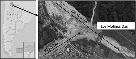
The case study is Los Molinos derivation Dam, located in the province of Jujuy, Argentina (UNC 2012). The dam is located on the river “Rio Grande”, upstream of the city of San Salvador de Jujuy and approximately 1 km downstream of the confluence with the Reyes River (Figure 1).
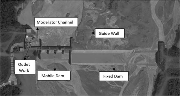
The derivation dam is composed of three discharge structures. On the left bank of the river there is a fixed weir (Fixed Dam, DF), which is separated from the mobile structures by a guide wall. The two mobile structures consist of a weir with four circular gates (Mobile Dam, DM) and a bottom discharger (or Moderator Channel, CM) regulated by two flat gates. Finally, on the right bank of the river is the water catchment structure (Figure 2).
Since the construction of Los Molinos dam the sediments transport have been affected. In the first years, an interruption of the sediment flow was generated from the upstream to the downstream sector.
This process led to the clogging of the reservoir and resulted in a generalized descent of the mobile bed downstream of the dam of approximately 9 m. This new configuration of the dam environment is different from the initial design conditions of the energy dissipation structures. Therefore, the structures began to operate inefficiently and local erosions were generated downstream of the structures on the right bank of the river.
To adapt the existing structures to the new configuration, modifications were proposed to the dissipation structures which consisted in modifying the dissipater type Gandolfo - Cotta of the mobile structures by ski jumps. The objective of these structures is to move the dissipation zone away from the foundation of the dam so that the erosions are produced far from the dam and do not compromise the stability of the dam.
As a complementary structure, to avoid stability problems, a concrete wall was designed downstream of the three discharge structures. The lower level of the wall was defined as a function of the maximum erosion obtained in this study, and the geotechnical characteristics of the river material.
Materials and methods
Experimental setup
The tests were carried out in the physical model of Los Molinos Dam (Jujuy, Argentina), which was designed to evaluate the hydraulic performance of the discharge structures designed to adapt the existing structures. The set up consists of a three-dimensional physical model (3D) with similarity of Froude, undistorted length scale (EL = 1: 65) with fixed margins, and moving bottom in the bed downstream of the dam.
The physical model includes the three discharge structures (Fixed Dock, Mobile Dock and Moderator Channel) with their control structures (gates). The domain of the model extends upstream of the dam, covering the approach sections of the Rio Grande and Reyes River with their confluence (approximately 1 000 m) and downstream the model extends about 500 m in the prototype. These distances were defined so that the imposed edge conditions do not affect the behavior of the flow in the erosion zone.
To define the geometry of the river in the area of approach to the dam, the cross-section method for rivers in regime was applied. This method allowed to determine width B, depth H of the cross-section, and the slope S as a function of a dominant flow (Farias, 2005).
To determine the dominant flow, a statistical criterion was applied, which is based on the assignment of a recurrence between 1.4 years and 2.33 years to this flow. A dominant flow of 600 m3/s was adopted, which corresponds to a recurrence of 2 years, and a width of 110 to 150 m.
To define the boundary conditions downstream of the dam, a numerical model 1D was developed using the HEC-RAS (USACE) program.
Mobile bed material
In a mobile bed physical model with sediment transport, the results depend on the granulometric distribution of the bed material.
Since it is impossible to achieve the complete similarity of the granulometric curve between the model and the prototype, a granulometry that best represents the physics of the processes involved must be selected to be used in the model (armoring, fluvial macro forms, etc.).
To represent the moving bed in the model, a kind of material with density and clastic characteristics similar to those of the prototype was used. Figure 3 shows the granulometric curve of the bed at 1:65 scale, which will be called the ideal curve.
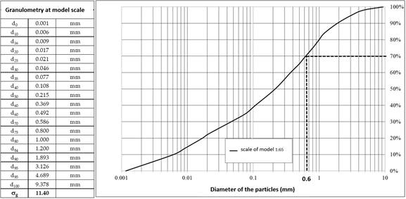
To go from the ideal curve to that used in the model, the following considerations were taken into account:
The bottom 35 percent of the "ideal" granulometric curve corresponds to cohesive sediments (diameters less than 75 microns). Therefore, this fraction of the granulometric curve cannot be represented in the physical model.
A minimal diameter of the granulometry of 0.6mm is adopted in order to avoid the generation of bottom “parasite” shapes, which would modify the bed roughness and would distort the similarity between the model and the prototype
The selected scale (1:65) allows to represent the upper fraction of the "ideal" curve, which includes diameters greater than d70. Table 1 shows that most of the empiric formulas that were developed use characteristic diameters included in this fraction of the curve (d85, d90 and d95).
Table 1 Parameters of the general formula of the erosion depth equation (see citations * in Mason & Arumugam, 1985).
| Formula N° | Reference | K | x | y | Z | d |
|---|---|---|---|---|---|---|
| 1 | Veronese - A (1937) * | 1.9 | 0.54 | 0.225 | 0 | |
| 2 | Damle - A (1966) * | 0.652 | 0.5 | 0.5 | 0 | |
| 3 | Damle - B (1966) * | 0.543 | 0.5 | 0.5 | 0 | |
| 4 | Damle - C (1966) * | 0.362 | 0.5 | 0.5 | 0 | |
| 5 | Chian Min Wu (1973) * | 1.18 | 0.51 | 0.235 | 0 | |
| 6 | Taraimovich (1978) * | 0.633 | 0.67 | 0.25 | 0 | |
| 7 | Machado - A (1982) * | 2.98 | 0.5 | 0.25 | 0 | |
| 8 | Sofrelec (1980) * | 2.3 | 0.6 | 0.1 | 0 | |
| 9 | INCYTH (1985) | 1.413 | 0.5 | 0.25 | 0 | |
| 10 | Martins - B (1975) * | 1.5 | 0.6 | 0.1 | 0 | |
| 11 | Lopardo (1987) | 0.798 | 0.5 | 0.5 | 0 | |
| 12 | Schoklitsch (1932) * | 0.521 | 0.57 | 0.2 | 0.32 | d90 |
| 13 | Veronese - B (1937) * | 0.202 | 0.54 | 0.225 | 0.42 | d50 |
| 14 | Egenberger (1943) * | 1.44 | 0.6 | 0.5 | 0.4 | d90 |
| 15 | Hartung (1959) * | 1.4 | 0.64 | 0.36 | 0.32 | d85 |
| 16 | Franke (1960) * | 1.13 | 0.67 | 0.5 | 0.5 | d90 |
| 17 | Kotoulas (1967) * | 0.78 | 0.7 | 0.35 | 0.4 | d90 |
| 18 | Zeller (1981) * | 0.88 | 0.686 | 0.686 | 0.372 | d95 |
| 19 | Chee y Padiyar (1969) * | 2.126 | 0.67 | 0.18 | 0.063 | d50 |
| 20 | Bisaz y Tschopp (1972) * | 2.76 | 0.5 | 0.25 | 1 | d90 |
| 21 | Chee y Kung (1971) * | 1.663 | 0.6 | 0.2 | 0.1 | d90 |
| 22 | Machado - B (1982) * | 1.35 | 0.5 | 0.3145 | 0.0645 | d90 |
Selection of the material of the moving bed in the model
The selection of the material of the moving bed is not trivial and is critical for reproducing the phenomenon of local erosion in the prototype.
Three different samples were analyzed, see Figure 4:
Sample 1: Sand with diameters between 1 and 2 mm
Sample 2: Sand and Gravel with diameters between 0.6 and 12 mm
Sample 3: Sand with diameters between 0.6 and 4mm
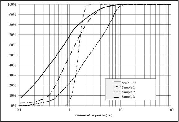
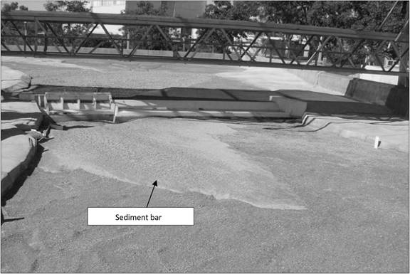
In the ideal granulometric curve it is observed that diameters d85 - d95 are in the range of 1.2 to 3.4 mm, the three samples analyzed have a fraction greater than 25% between these limits. Therefore, it could be considered that the three samples may be appropriate to reproduce the phenomenon of local erosion. As a consequence of this erosion, it is expected that first, that downstream a sediment bar may form with the bed material. Second, it is also expected to observe segregation of the granulometry without reaching armoring.
Calibration tests were carried out to determine which of the three samples is the one that best reproduces the phenomenology. The observations in the three samples were as follows. In sample 1 the sedimentation bar was not formed downstream of the erosion zone, and erosion continued indefinitely over time. Therefore, the erosive process did not stabilize. Consequently, it was considered that this sample did not represent the phenomenon. In sample 2 the sediment bar was formed and the erosion stabilized; however, it produced an armor in the downstream slope and in the sediment bar with a diameter of approximately 8 to 12 mm, equivalent to 520 and 780 mm in the prototype. The material of this size in the prototype is a small proportion (less than 5%). This is the reason why it was considered that this type of armoring could not be formed. Thus, sample 2 was rejected since it was not representative of the phenomenon. In sample 3 the sediment bar was formed and the erosion stabilized in addition, there was a segregation of the sediments in the downstream slope, and in the sediment bar with an average diameter of 4 mm, equivalent to 260 mm in the prototype (Figure 5). It was considered that this sample was the one that best reproduced the physical phenomenon, and was the one chosen to carry out the erosion tests in the model.
It is concluded that, regarding the case analyzed, the stabilization of the erosion depends on the formation of the sediment bar, and it depends on the transport of sediments. Therefore, the dimensions and shape of the local erosion is a function of the hydraulic and sediment characteristics as well as their granulometric distribution. Interestingly, in this work the final erosion is a function of the granulometric curve unlike Mason and Arumugam (1985) and Heng et al. (2013) where the sediment bar formation is not considered.
Modeled hydraulic conditions
Test 1. Flow = 900 (m3/s) spilling through the moderator channel and the mobile dam.
Test 2. Flow=3200 (m3/s) spilling through the fixed dam.
Test 3. Flow=4200 (m3/s) spilling through the moderator channel, the mobile dam, and the fixed dam.
Test 4. Flow=1600 (m3/s) spilling through the moderator channel, the mobile dam, and the fixed dam.
Test 5. Flow=600 (m3/s) spilling through the moderator channel and the mobile dam.
Experimental methodology
The erosion zone was surveyed with an optical level in three profiles parallel to the structure but perpendicular to the flow. Profile 1 was measured next to the dam, profile two was taken at the maximum depth of the erosion pit, and profile three was obtained on the sediment bar.
Also, the erosion surface was measured (Figure 6a) using a digital camera (Microsoft, 2010) which allows the acquisition of planimetric information with high spatial resolution. With this information a digital elevation model was generated (DEM, Figure 6b) similar to Pagot et al. (2014).
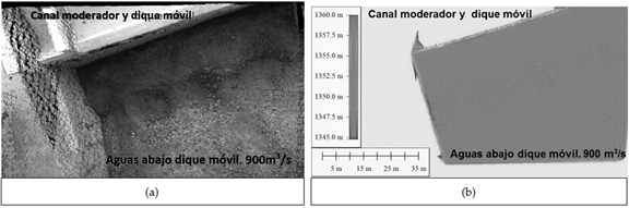
Figure 6 (a) Optical image of the erosion downstream of the mobile dam using Kinect, y (b) Digital Elevation Model.
This survey technique has the advantage of acquiring high spatial resolution data remotely without being in contact with the surface.
To ensure that the erosion pit reaches a state of dynamic quasi-equilibrium, erosion monitoring was carried out while the tests at 12 control points were carried out. During the first 90 minutes of the test, measurements were taken every 15 minutes and then every 30 minutes until the erosion was stabilized. It was considered that when three consecutive measurements did not differ significantly, this equilibrium state was reached.
In addition, to locate the zones of maximum velocity and the transversal distribution of the flow, the entrance velocities to the structures were measured by PTV technique (Velocimetry by particle tracking). The velocimetry technique by particle tracking allows to obtain the instantaneous and average velocity fields, trajectory lines, and average trajectory lines. To analyze the images, the PTVLab software (Patalano, 2017) was used.
Empirical Estimates of the Maximum Depth of Erosion (h s )
There are numerous investigations that present semi-empirical formulations that allow to determine the maximum depth of erosion based on energetic considerations of the flow and the characteristics of the material of the bed such as typical diameters.
Below are the equations used in this work to determine the maximum depth of erosion. These equations were classified into three groups according to the parameters that intervene in each of them:
Group I - Equations that express the maximum depth of
erosion (
The general formula of this group of equations is as follows:
where:
Formulas 1 to 11 have zero exponent of the characteristic diameter. Therefore, these expressions do not take into account the diameter of the sediments to determine the maximum depth of erosion pit.
Within this group the formula proposed by the I.D.I.H is included:
Formula 23 - I.D.I.H. (1990): h 𝑠 =2.6662𝑞 𝐻 −0.5 +0.3291𝐻
Group II - These equations contemplate in addition to the variables
Formula 24- Jaeger (1939):
Formula 25 - Martins - A (1973):
where:
The discharge Q can be substituted for q because it is assumed that this expression may be applicable for large flow sheets.
Formula 26 - Mason (1984):
Group III - These equations also consider the angle at which the jet hits the water (β).
Formula 27 - Mikhalev (1960):
Formula 28- Rubinstein (1963):
Formula 29 - Mirskhulava - (1967):
The 29 formulas considered are semi-empirical and were calibrated from experimental data obtained from physical models or erosion values observed in the prototype.
To estimate the specific flows (q) that each of the structures spill, two aspects were considered. First, the H-Q curves corresponding to each structure, and second the flow was distributed uniformly along the width of the structure. The height of energy (H) was obtained by adding the geometric difference between the level upstream and the restitution to the speed energy in the section in which the measurement of the levels was carried out.
where,
|
geometrical difference between the upstream level and the level of restitution |
|
average speed in the upstream section |
To assign values to the characteristic diameters that intervene in the formulas the granulometric curve of the bed was used (d95=0.130m; d90=0.123m; d85=0.116m y d50=0.068m).
Results
Experimental studies
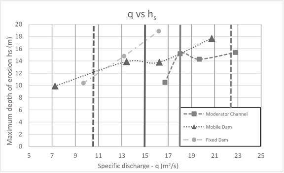
The maximum depth of erosion (
In principle, it is expected that as the specific flow rate (q) and the power
height (H) increase, the maximum depth of erosion (
To explain the lack of monotonous behavior, two hypotheses were formulated:
Hypothesis1: The lack of monotonous behavior is produced by a change in the flow direction upstream of the structures. In the tests carried out in the physical model, a change in the flow direction was observed when the water drained by the Fixed Dam.
Hipótesis2: The behavior observed in Figure 9 and Figure 10 is due to a change in the H-Q relations of the Moderator Channel and the Mobile Dam. When the water level exceeds the height of the gates they begin to function as an orifice. This is the reason why there is a change in the H-Q relations.
Approach flow
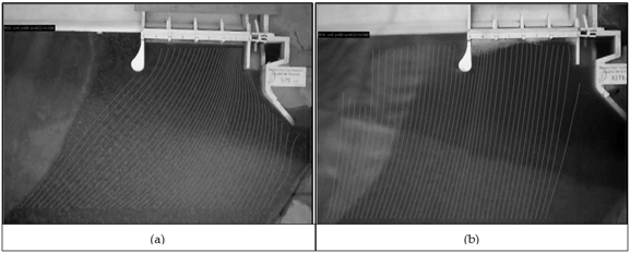
Applying the PTV technique (Patalano, 2017) it was observed that, when the water drains only by the Mobile Dam and the Moderator Channel, the flow current lines enters obliquely (Figure 7a). When the water drains through the three structures, the current lines upstream of the dam enter perpendicular to the dam (Figure 7b).
Discharge curves
To quantify the discharges of the structures, their height-flow curves (H-Q) were obtained. The fitting was made with experimental data obtained from the physical model for each of the structures. Figure 8 (a) shows the height-discharge curve of the Mobile Dam and in Figure 8 (b) that of the Moderator Channel. It can be seen that the Mobile Dam begins to work as an orifice when the height above the landfill is approximately 5.4 m and the Moderator Channel for a height of 6 m.
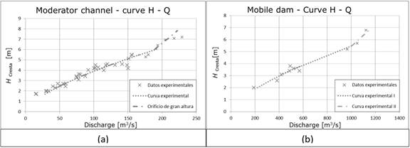
Figure 9 shows, in a dashed line, the specific flow corresponding to Hypothesis 1 and in a continuous line the flow corresponding to Hypothesis 2. It is observed that the change in the flow direction upstream of the structures (Hypothesis 1) has no significant influence on the unexpected behavior of the relationships (q-hs) and that the specific flow corresponding to Hypothesis 2 (change in the height-discharge relationships), for the two structures, is in the range of flow rates in which a different behavior than expected was observed. Then, it is concluded that the unexpected behavior between the discharge vs. erosion depth relationships can be explained by the change in the H-Q relationships.
In Figure 10 it is observed that
the change in slope in the relationships
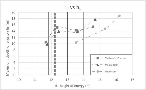
Empirical estimates
The erosion values (
Next, the experimental results were compared with the estimates. Figure 11 (a), (b) and (c) present the scatter diagrams of the experimental erosion depth versus estimated erosion for the Moderator Channel, the Mobile Dam, and the Fixed Dam, respectively. It was observed that no formula worked satisfactorily for the three structures.
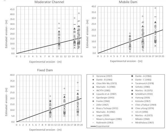
Figure 11 Comparison diagram between experimental erosions and empirical estimates, (a) Moderator Channel, (b) Mobile Dam and (c) Fixed Dam.
Figure 12 shows a BOX-PLOT graph in which the results for the three structures are presented. It can be seen that the experimental result for the Moderator Channel is close to the second quartile (Q2) and that the experimental values corresponding to the Mobile Dam and the Fixed Dam are located close to the third quartile (Q3). It is concluded that the maximum depth of erosion not only varies with the sedimentological conditions, which in this case remain constant for the three structures, but also with the hydraulics of each work in particular.
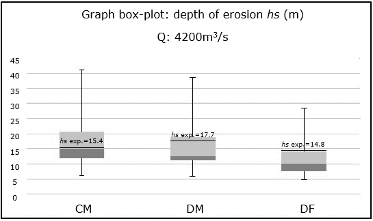
Figure 12 BOX-PLOT graph of Chanel Moderator, Mobile Dam and Fixed Dam for a flow rate of 4 200 m3/s.
Table 2 shows the percentage relative differences between the maximum erosions measured in the physical model and those estimated with the different empirical formulations for each of the structures and each of the scenarios tested. The formulas that were best adapted to the conditions tested for the three discharge structures were those proposed by Zeller (1981) and Machado B (1982). Those that best adapted to the experimental measurements made in the Moderator Channel were Rubinstein (1963), Lopardo (1987), Mirskhulava (1967), Zeller (1981), Machado B (1982) and INCYTH (1985); for the Mobile Dam were Veronese (1937), Sofrelec (1980), Machado (1982), Mason and Arumugam (1985), IDIH (1990), Jaeger (1939) and Zeller (1981) and for the Fixed Dam were Machado B (1982), Veronese (1937), Zeller (1981), Mason and Arumugam (1985) and Sofrelec (1980).
Table 2 Percentage difference between the empirical estimates and experimental erosion for the CM, DM and DF.
| Moderator channel | Mobile dam | Fixed dam | ||||||||||
|---|---|---|---|---|---|---|---|---|---|---|---|---|
| Discharge total (m3/s) | 600 | 900 | 1600 | 4200 | 600 | 900 | 1600 | 4200 | 1600 | 4200 | 3200 | |
| Erosion Experimental hs (m) | 10.5 | 15.2 | 14.3 | 15.4 | 9.9 | 13.9 | 13.8 | 17.7 | 10.4 | 14.8 | 18.9 | |
| Formula | Percentage difference between the empirical estimates and experimental erosion (%) | |||||||||||
| 1 | Veronese (1937) | 44 | 5 | 19 | 22 | -3 | -2 | 12 | 1 | 12 | -4 | -15 |
| 2 | Damle - A (1966) | -13 | -36 | -26 | -23 | -39 | -39 | -30 | -36 | -28 | -37 | -44 |
| 3 | Damle - B (1966) | -28 | -47 | -38 | -36 | -49 | -50 | -42 | -46 | -40 | -48 | -53 |
| 4 | Damle - C (1966) | -52 | -64 | -59 | -57 | -66 | -66 | -61 | -64 | -60 | -65 | -69 |
| 5 | Chian Min Wu (1973) | -16 | -39 | -30 | -29 | -42 | -42 | -35 | -41 | -33 | -44 | -50 |
| 6 | Taraimovich (1978) | -26 | -46 | -37 | -35 | -55 | -51 | -43 | -47 | -47 | -52 | -57 |
| 7 | Machado - A (1982) | 114 | 56 | 77 | 81 | 50 | 47 | 67 | 50 | 71 | 45 | 27 |
| 8 | Sofrelec (1980) | 52 | 10 | 25 | 27 | -2 | 1 | 15 | 5 | 12 | -4 | -15 |
| 9 | INCYTH (1985) | 2 | -26 | -16 | -14 | -29 | -30 | -21 | -29 | -19 | -31 | -40 |
| 10 | Martins - B (1975) | -1 | -28 | -19 | -17 | -36 | -34 | -25 | -32 | -27 | -37 | -44 |
| 11 | Lopardo et al. (1987) | 6 | -22 | -9 | -6 | -26 | -26 | -14 | -21 | -12 | -23 | -32 |
| 12 | Schoklitsch (1932) | -21 | -42 | -34 | -33 | -48 | -47 | -39 | -45 | -40 | -48 | -54 |
| 13 | Veronese (1937) | -53 | -66 | -61 | -60 | -68 | -68 | -63 | -67 | -63 | -69 | -72 |
| 14 | Egenberger (1943) | -7 | -31 | -19 | -15 | -40 | -36 | -25 | -30 | -27 | -34 | -40 |
| 15 | Hartung (1959) | -11 | -34 | -23 | -20 | -44 | -40 | -30 | -34 | -33 | -40 | -45 |
| 16 | Franke (1960) | -31 | -48 | -39 | -35 | -58 | -53 | -44 | -47 | -48 | -52 | -56 |
| 17 | Kotoulas (1967) | 191 | 117 | 153 | 167 | 73 | 93 | 129 | 118 | 111 | 93 | 78 |
| 18 | Zeller (1981) | 20 | -9 | 9 | 18 | -28 | -18 | 0 | -3 | -8 | -13 | -18 |
| 19 | Chee y Padiyar (1969) | 147 | 81 | 108 | 116 | 50 | 63 | 89 | 76 | 78 | 57 | 42 |
| 20 | Bisaz y Tschopp (1972) | 90 | 39 | 58 | 61 | 30 | 30 | 48 | 34 | 50 | 28 | 13 |
| 21 | Chee y Kung (1971) | 83 | 34 | 53 | 58 | 18 | 23 | 41 | 30 | 38 | 19 | 7 |
| 22 | Machado - B (1982) | 30 | -5 | 9 | 11 | -9 | -10 | 3 | -7 | 5 | -10 | -21 |
| 23 | I.D.I.H (1990) | 61 | 17 | 31 | 35 | -4 | 2 | 17 | 9 | 10 | -5 | -15 |
| 24 | Jaeger (1939) | 43 | 7 | 22 | 44 | 0 | 1 | 15 | 20 | 17 | 15 | -4 |
| 25 | Martins - A (1973) | -28 | -45 | -35 | -13 | -54 | -51 | -41 | -29 | -44 | -35 | -47 |
| 26 | Mason y Arumugan (1985) | 45 | 6 | 19 | 30 | -7 | -3 | 10 | 7 | 7 | -2 | -15 |
| 27 | Mikalev (1960) | 47 | 9 | 27 | 37 | -57 | -43 | -31 | -31 | -61 | -63 | -65 |
| 28 | Rubinstein(1963) | 7 | -21 | -9 | -3 | -35 | -32 | -20 | -22 | -33 | -32 | -40 |
| 29 | Mirskhulava (1967) | 20 | -10 | 5 | 13 | -87 | -83 | -79 | -34 | -49 | -63 | -62 |
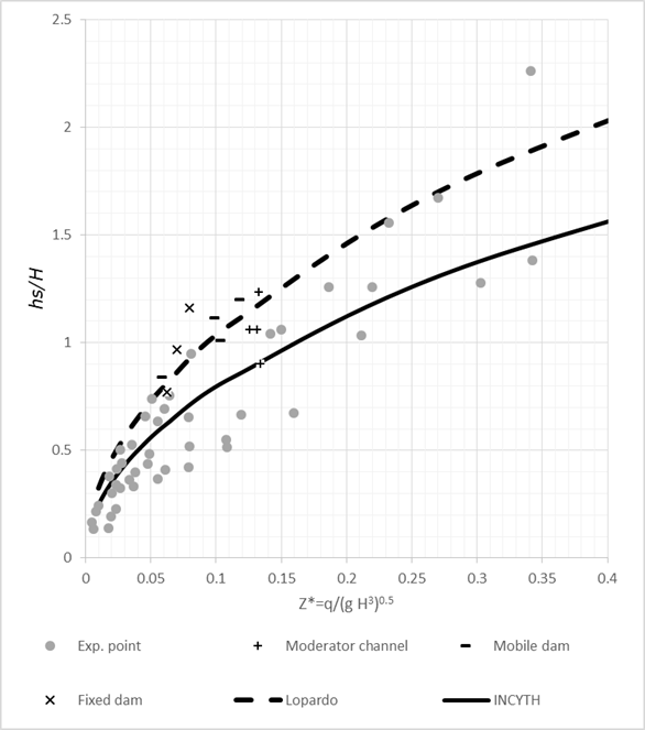
Finally, the experimental results observed in this study are compared with
those presented in similar cases using the graph by Lopardo (2005). In this graph, the main variables are
related in a nondimensional way. Figure
13 shows the curves corresponding to the expression proposed by
INCYTH, together with experimental points of erosions in prototype works
(Ptos exp.), the envelope curve given by the design expression proposed by
Lopardo, and the results obtained in this work for each of the structures.
It is observed that the points measured in this work are close to the
envelope proposed by Lopardo and in some cases
Conclusions
In the calibration stage "Selection of the granular material of the mobile bed" it was observed that the erosions depend on the formation of the sediment bar downstream of the erosion pit and the formation of the bar depends on the characteristic diameters of both the particles and the granulometric curve.
When the jet of water hits the bed, a great dissipation of macro-turbulent energy is generated, which initiates the local erosion process. The bottom material is removed, placed in suspension, and transported downstream where the flow reduces its energy, and therefore its transport capacity.
Finally, the sedimentation of the larger particles takes place, and initiates the formation of the sediment bar. The latter contributes to stabilize the erosions, reaching lower depths than those that would occur without the formation of the sediment bar, due to two effects. First, it increases the level of restitution in the energy dissipation zone. This reduces the value of H and increases the height of the water in the impact zone hr. Second, it raises the level of the bed downstream of the erosion pit. Therefore, for the sediments to come out of the erosion pit they must be raised to a larger height.
Regarding the "analysis of experimental results", it is concluded that, for structures of low height regulated by gates, the relations between q and H with the maximum depth of erosion (hs) vary with the discharge law (H-Q) of the structures. A large dispersion was observed in the results when erosions (hs) were calculated with "empirical formulas". The application of these formulas must be limited to preliminary estimates to obtain an order of magnitude of the potential erosions.
When only empirical expressions are used, formulas that have been calibrated for hydraulic and sedimentological conditions similar to those used in this work should be applied. In this study, the formulas that showed the best behavior for the conditions tested are those by Zeller (1981) and Machado-(1982).
Ahmed-Amin, A. M. (2015). Physical model study for mitigating local scour downstream of clear over-fall weirs. Ain Shams Engineering Journal (Egypt), 6, 1143-1150. [ Links ]
Farias, H. D. (2005). Geometría hidráulica de ríos de llanura. Enfoques analíticos considerando la influencia de las márgenes (CD-ROM). Segundo Simposio Regional sobre Hidráulica de Ríos, Neuquén, Argentina. [ Links ]
Fuentes, R. (2002). Modelos hidráulicos: teoría y diseño. Santiago, Chile. [ Links ]
Google. (2012) Google Earth (website). Recuperado de http://earth.google.com/ [ Links ]
Heng, T., Tingsanchali, T., & Suetsugi, T. (2013). Prediction formulas of maximum scour depth and impact location of a local scour hole below a chute spillway with a flip bucket, WIT Transactions on Ecology and The Environment, 172 (River Basin Management VII), 251-262. [ Links ]
Lopardo, R. (2005). Erosión local aguas debajo de estructuras hidráulicas. Curso sobre hidráulica experimental aplicada a estructuras. Ciudad Real, España. [ Links ]
Mason, P., & Arumugam, K. (1985). Free jet scour below dams and flip buckets. Journal of Hydraulic Engineering, 111(2), 220-235. [ Links ]
Microsoft. (2010). Kinect. Recuperado de http://idav.ucdavis.edu/~okreylos/ResDev/Kinect/index.html [ Links ]
Pagot, M., Sánchez-Aimar, E., Vaca, P., Nellino, N., Guillén, N., Hillman, G., & Rodríguez, A. (2014). Técnica digital para medición de erosión en modelos físicos. Revista Facultad de Ciencias Exactas, Físicas y Naturales (UNC), 1(2), 35-40. [ Links ]
Patalano, A., García, C. M., y Rodríguez, A. (2017). Rectification of Image Velocity Results ( RIVeR ): A simple and user-friendly toolbox for large scale water surface Particle Image Velocimetry ( PIV ) and Particle Tracking Velocimetry (PTV). Computers & Geosciences, 109, 323-330. DOI: 10.1016/j.cageo.2017.07.009 [ Links ]
UNC, Universidad Nacional de Córdoba. (2012). Proyecto y construcción del modelo físico tridimensional del dique derivador Los Molinos, provincia de Jujuy. (Informe Técnico). Córdoba, Argentina: Universidad Nacional de Córdoba. [ Links ]
Received: March 09, 2017; Accepted: November 08, 2018
 Este es un artículo publicado en acceso abierto bajo una licencia
Creative Commons
Este es un artículo publicado en acceso abierto bajo una licencia
Creative Commons
