


Serviços Personalizados
Journal
Artigo
 texto em
  Espanhol (pdf)
 Artigo em XML
 Referências do artigo
 Enviar este artigo por email
Indicadores
-
 Citado por SciELO
 -
 Acessos
Links relacionados
-
 Similares em
SciELO
Similares em
SciELO
Compartilhar

 Permalink
Tecnología y ciencias del agua
versão On-line ISSN 2007-2422
Tecnol. cienc. agua vol.9 no.1 Jiutepec Jan./Fev. 2018 Epub 24-Nov-2020
https://doi.org/10.24850/j-tyca-2018-01-01
Articles
Regional analysis to estimate design precipitation in the Mexican Republic
1Universidad Nacional Autónoma de México, Ciudad de México, México, rdominguezm@iingen.unam.mx
2Universidad Nacional Autónoma de México, Ciudad de México, México, ecarrizosae@iingen.unam.mx
3Universidad Nacional Autónoma de México, Ciudad de México, México, gfuentesm@iingen.unam.mx
4Universidad Nacional Autónoma de México, Ciudad de México, México, marganisj@iingen.unam.mx
5Universidad Nacional Autónoma de México, Ciudad de México, México, josnayar@iingen.unam.mx
6Universidad Nacional Autónoma de México, Ciudad de México, México, andresgalvant@gmail.com
In this paper, we present a regional analysis of maximum daily rainfall recorded by more than 2000 rain gauges in the Mexican Republic. The results allow to estimate design storms for any watershed in Mexico reliably. For the analysis, we clustered 59 regions based on the terrain morphology and the way they are affected by extreme weather. Additionally, the annual maximum daily precipitations were divided by their respective mean, resulting in samples with mean equal to 1 and standard deviation equal to the variation coefficient. To verify the homogeneity for each zone, the Fisher test was considered, but taking in to account that such test is not strictly applicable to extreme distributions, it was also proposed to generate synthetic series to validate the variation coefficient behavior of the sample. To estimate the design storms, characteristic hyetographs were obtained for total durations higher or lower than one day.
Keywords Regional analysis; daily annual maximum rainfall; Design storm; Duration; Return period; Convectivity
En este artículo se presenta un análisis regional de las lluvias diarias máximas anuales registradas en más de 2000 estaciones de la república mexicana.Los resultados permiten estimar de manera confiable las tormentas de diseño para cualquier cuencaen México.Para el análisis se agruparon59 regiones de acuerdo con el relieve del terreno y la forma en la que los fenómenos hidrometeorológicos extremos lo afectan; además, se dividieron las precipitaciones diarias máximas anuales de cada estación entre su promedio respectivo, de manera que en todos los casos la media resulta 1 y la desviación estándar igual al coeficiente de variación. Para verificar la homogeneidad de cada zona se consideró la prueba de Fisher, pero tomando en cuenta que dicha prueba no es estrictamente aplicable a distribuciones extremas; se planteó además la generación de series sintéticas para validar el comportamiento de los coeficientes de variación de las muestras.Para la estimación de las tormentas de diseño se considera la conformación de hietogramas característicos para duraciones totales menores o mayores que un día.
Palabras clave análisis; regional; lluvias diarias máximas anuales; tormenta de diseño; duración; periodo de retorno; convectividad
Introduction
In Mexico, there is information of daily rains measured in more than 5000 stations. The analysis of these records shows that in many stations the available data are scarce, so that the statistical analyses performed individually are not reliable (for example, CONAGUA uses only 1788 stations for the calculation of climatological normals) (CONAGUA, 2015). In the case of pluviographic records, the situation worsens, both because of the limited number of stations and the quality and accessibility of that information.
Numerous attempts have been made to estimate rainfall associated to different durations and return periods (Conde, Vita, Castro & López, 2014, SCT, 1990), but an individual analysis is carried out, station by station, which often results in inconsistencies in the results.
In the last years and in different countries, there have been extensive studies on the regional analysis of rainfall frequencies, some of which are supported by the L moments technique (Escalante & Reyes, 2005), as well as by principal components analysis (Gellens, 2002; St-Hilaire et al., 2003; Wotling, Bouvier, Danloux & Fritish, 2000), the use of clustering techniques (cluster analysis) for regional grouping, technic of year-seasons, the Dalrymple method and quantile analysis and computation of fractiles (Dalrymple, 1960; Conleth,1988, Buishand, 1991; Cunnane, 1988; Gellens, 2002; Yang et al., 2010).Some authors propose to use the general distribution of extreme values (GEV) for the analysis of extreme rainfall for different durations (Rossi, Fiorentino & Versace, 1984; Gellens, 2002; St-Hilaire et al., 2003); Koutsoyiannis (2009a and b) indicates in his case study that a type II extreme value function is better suited than Gumbel functions to precipitation records even with few data.
Berndtsson and Niemczynowicz (1988) conducted a state-of-the-art review of the various factors involved in precipitation analysis; they emphasize the time and space scales to be used depending on the scope of the hydrological problem; the two types of precipitation analysis stand out: at a single point level to obtain the period of return of rains with different characteristics, and the analysis of the simultaneity of the precipitations considering different sites to make regional estimates.
In Mexico, storm regionalization studies have been carried out in the Valley of Mexico basin (Cortés, 2003). Guichard & Domínguez (1998) in their study of regionalization of basins of the Upper Grijalva consider several studies on the factors of reduction by area, by period of return and by duration (Bell, 1969; Chen, 1983).
Rainfall regionalization studies using the General Distribution of Extreme Values carried out in San Luis Potosí, Sinaloa, Mexico (Campos-Aranda, 2008 and 2014) are highlighted. In addition to the regional estimation of convectivity factors (Baeza, 2007), precipitation maps for different periods of return and durations have been made in the Mexican Republic (Domínguez et al.; Secretaría de Comunicaciones y Transportes, 1990); also, the influence of regionalization on the estimation of daily maximum precipitation (Escalante and Amores, 2014), the regionalization of precipitation with bivariate functions and maximum entropy (Escalante and Domínguez, 2001), climate change at regional scale in precipitation and temperature (Magaña & Galván, 2010).
In this work, regional analyses are carried out based on information from 2293 rain gauges, which allows the estimation of design rainfall (associated with different return periods) for different durations; a procedure using synthetic series for the validation of homogeneous zones is also presented that compares historical and synthetic coefficients of variation. In making the regional analysis, spatially consistent results are achieved, avoiding the inconsistencies that are obtained when analyzing each station individually.
In relation to rains with duration less than one day, results from Baeza and Mendoza (Baeza, 2007, Mendoza, 2001) are taken; they used the original information compiled by the Ministry of Communications and Transportation (Secretaría de Comunicaciones y Transportes, 1990), and also from the former Ministry of Hydraulic Resources (mainly the Papaloapan Commission bulletins), but they managed it regionally using the concept of "convectivity" based on the theory developed by Chen (1983) and considering the topographical conformation and climatological environment of each season. The results obtained allow to estimate design logs for different time intervals and different total storm durations, using the alternating block method (Chow, Maidment & Mays, 1988), for any basin of the Republic.
Methodology
Data from a total of 2293 stations in the Climate Computing Project database (CLICOM) (Figure 1) were analyzed. Table 1 shows the number of stations considered in each state as well as the corresponding average number of record years.
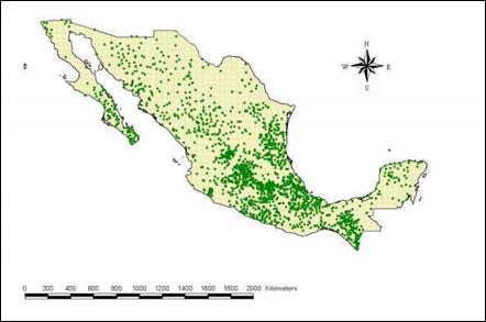
Table 1 Stations selected by State
| State | Number of stations by 2010 | *Average recorded years | State | Number of stations by 2010 | *Average recorded years |
|---|---|---|---|---|---|
| Aguascalientes | 50 | 35.18 | Morelos | 44 | 33.68 |
| Baja California Norte | 37 | 32.68 | Nayarit | 25 | 30.32 |
| Baja California Sur | 72 | 33.03 | Nuevo León | 55 | 31.27 |
| Campeche | 42 | 32.64 | Oaxaca | 129 | 29.93 |
| Chiapas | 109 | 33.55 | Puebla | 98 | 38.56 |
| Chihuahua | 58 | 30.84 | Querétaro | 34 | 32.24 |
| Coahuila | 28 | 33.76 | Quintana Roo | 20 | 30.8 |
| Colima | 17 | 46.76 | San Luis | 103 | 32.23 |
| Ciudad de México | 30 | 28.9 | Sinaloa | 51 | 31.1 |
| Durango | 83 | 42.39 | Sonora | 79 | 32.75 |
| Estado de México | 114 | 27.7 | Tabasco | 42 | 35.79 |
| Guanajuato | 108 | 37.86 | Tamaulipas | 109 | 30.28 |
| Guerrero | 125 | 39.75 | Tlaxcala | 20 | 32.6 |
| Hidalgo | 66 | 44.2 | Veracruz | 190 | 31.1 |
| Jalisco | 180 | 39.74 | Yucatán | 30 | 29.97 |
| Michoacán | 93 | 34.37 | Zacatecas | 51 | 30.08 |
| Total | 2293 | 33.94 |
For the selection of the 2293 stations it was verified that they fulfilled the following requirements
Stations operating for at least 20 years and with the complete information in that recording period
In the case of the central and southern areas of the country, stations were included in which the missing data correspond to the dry season. In the northwest, due to the presence of intense rains in the winter season, only stations with full registration were included
For each of the stations the annual maximum daily values were obtained and the statistics calculated were: mean, standard deviation, coefficient of variation (CV), besides the maximum and minimum values. The analysis of these statistics allowed the debugging of values that at first seemed illogical (on the one hand, very small values or even zero for the maximum precipitations in a whole year and on the other very large values, on the order of four times the mean). In the case of very large values, the original log sheets were consulted with the help of the Superficial Water Management and River Engineering (GASIR) and, according to the results of that query, the incorrect ones were eliminated.
With the values cleared and considering both the coefficients of variation and the topographic conformation, homogeneous regions were defined from the point of view of the annual maximum daily precipitation, considering that, if in a region, the coefficients of variation are similar and the annual maximum values of each station are modulated by dividing them by their mean, the modulated samples will have a mean of 1 and a similar standard deviation. To test the hypothesis of homogeneity among the samples thus obtained, Fisher's test is traditionally used (Domínguez et al., 2014), but considering that the maximum values do not correspond to a normal probability distribution, a new procedure is proposed in this work to verify the hypothesis that the historical samples come from a population characterized by the distribution function adjusted to the enlarged sample. For this, synthetic series are generated and the CV of a set of samples with the same size as the historical ones, obtained from the adjusted distribution function calculated. The region is considered homogeneous if the range of simulated CV includes all the historical CV (Domínguez, Bouvier, Neppel & Niel, 2005).
The homogeneous samples obtained for each region will then be made up of much more values than those corresponding to each station considered individually, so that the results obtained by adjusting them to a probability distribution function will be much more reliable and robust.
Relation precipitation-duration-return period.
Estimates for storm durations less than 1h
The estimation of design flow rates for small or medium watersheds requires knowing the average rainfall associated with durations less than one day, that is, obtaining the curves precipitation- duration-return period.
Chen (1983) conducted studies on rainfall for different return periods supported by studies generated by USBW in the Paper No. 40 (TP 40), and obtained a generalized intensity-duration-return period formula for any location in the U.S. According to Chen's study, it is required to obtain rainfall for a 10-year return period for both 1 hour (P1 10) and 24 hours (P24 10), and for a 100-year return period, The rain height for 1 hour (P1 100). With these data, the ratios R = (P1 T / P24 T) and "X" = (P1 10/P1 100) are obtained. In addition, he found that the R ratio that relates the relationship of rain height to duration varies between 10% - 60% depending on the geographic location and that is probably independent of the return period; also found that the ratio X, rainfall height with the frequency seems to be independent of the duration and varies between the ranges of 1.33 to 1.63. These relationships were used for the construction of equation 1 with which the precipitation can be calculated for any duration and return period.
Valid for T ≥ 1 year and 5 min ≤ t ≤ 24 h, where
Baeza (2007), considers that in Mexico there is sufficient rainfall information to estimate the precipitation associated with a duration of 24h and any return period with greater precision than that obtained using the ratio X = P1 100/P 1 10 that proposes Chen. Baeza concentrates then on the analysis for the Mexican Republic of the factor R = P1 T / P24 T which he calls the "convectivity factor", which, on the contrary, is difficult to estimate with good precision given the scarcity of rainfall data available in Mexico. For this purpose, it uses the original information compiled by the Ministry of Communications and Transport (Secretaría de Comunicaciones y Transportes, 1990), as well as data recorded in bulletins of the then Ministry of Hydraulic Resources (mainly the Bulletins of the Papaloapan Commission). He handles it regionally using the concept of "convectivity" when considering the topographical conformation of the environment of each station and its relationship with the predominant meteorological phenomena in each zone.
Estimates for durations greater than one day
Also, and working with the same regions, average annual maximums are obtained for durations of 2, 3, ..., 30 days and their relationship with those of 1 day, for each of the 2293 stations studied. By averaging these relationships within each region factors are determined that allow a reliable estimate of the average precipitation associated with durations of up to 30 days from those obtained for one day.
Results
Capturing and debugging information
Stations with at least 20 years of complete records were reviewed. Table 1 shows the number of stations selected as well as the average number of years of registration for each state of the Republic. Table 2 shows, for example, the case of Durango; the values that seemed extremely large were marked with blue and with red those that were eliminated when it could be verified in the original registry, provided by the GASIR, that these are indeed capture errors; additionally, the minimum values that appear illogical (typically null values or only a few millimeters in rainy zones) are shown, marked with yellow.
Table 2 Table with corrections for Durango.
| Year | Station | |||||||||||||
|---|---|---|---|---|---|---|---|---|---|---|---|---|---|---|
| 10001 | 10002 | 10003 | 10004 | 10012 | 10014 | 10016 | 10018 | 10020 | 10021 | 10028 | 10029 | 10030 | 10033 | |
| 1975 | 25 | 40 | 81 | 20 | 38 | 48 | 45 | 17 | 57 | 70 | 53 | 77 | ||
| 1976 | 35.5 | 60 | 136.8 | 20 | 48 | 144 | 42 | 32 | 53 | 54 | 25.5 | |||
| 1977 | 40 | 125 | 21.1 | 52.2 | 40 | 138 | 40 | 33 | 45 | |||||
| 1978 | 40 | 62 | 88 | 28.8 | 28.5 | 36 | 84 | 53 | 60.3 | 31 | 33 | 32 | ||
| 1979 | 11.4 | 170 | 37 | 55 | 89 | 206 | 40 | 43 | 35 | 20.5 | ||||
| 1980 | 8.9 | 45 | 50 | 37.5 | 57 | 43 | 35.5 | 106 | 46 | 47 | 38 | 28 | ||
| 1981 | 30 | 54.2 | 27 | 39 | 65 | 40.8 | 57 | 20 | 32.5 | 70 | 60 | |||
| 1982 | 31.7 | 45 | 70 | 32 | 75.1 | 31.6 | 34 | 34.5 | 34 | 62.5 | ||||
| 1983 | 75 | 48 | 105 | 26.2 | 82.5 | 44.8 | 117 | 24 | 36 | 56.5 | 53 | |||
| 1996 | 38 | 66 | 75.4 | 50 | 21 | 33.5 | 56 | 35 | ||||||
| 1997 | 28 | 30 | 97 | 86.5 | 41.5 | 280 | 89 | 33 | 71.5 | 24 | 20 | |||
| 1998 | 37.5 | 34 | 40.4 | 57.3 | 29 | 41.5 | 40 | 32.4 | ||||||
| 2001 | 25 | 26 | 28.5 | 14 | 34 | 34.2 | 22.5 | 28.1 | ||||||
| 2002 | 65 | 32.8 | 33 | 28 | 40 | 86 | 17.8 | 56 | 46 | 31.4 | ||||
| 2003 | 60 | 35 | 55.7 | 40 | 43 | 71.9 | 60 | 32 | 42.1 | |||||
| 2004 | 72 | 152 | 57.5 | 21 | 70 | 75.5 | 77.3 | 34.5 | 36.1 | |||||
| 2005 | 52.5 | 68.7 | 54.8 | 45.4 | 29.5 | 60 | 74 | 22.9 | 50.5 | 20.4 | ||||
| 2006 | 40 | 53 | 29.5 | 61.5 | 22 | 64 | 50 | 48 | 36.8 | |||||
| 2007 | 71.2 | 50 | 40 | 50 | 52.5 | |||||||||
| 2008 | 59.2 | 49.4 | 60 | 52 | 37.5 | 40 | ||||||||
| 2009 | 60 | 32.5 | 60 | |||||||||||
| 2010 | 30 | 81 | 60 | |||||||||||
| Mean | 40.234 | 48.135 | 88.314 | 37.414 | 48.019 | 52.655 | 40.679 | 93.649 | 40.097 | 42.979 | 45.125 | 40.784 | 44.270 | 54.979 |
| Std. Dev. | 15.505 | 20.627 | 35.420 | 15.520 | 14.359 | 18.617 | 43.523 | 42.510 | 18.140 | 15.359 | 16.327 | 11.247 | 18.327 | 48.342 |
| Coef. of Var. | 0.385 | 0.429 | 0.401 | 0.415 | 0.299 | 0.354 | 1.070 | 0.454 | 0.452 | 0.357 | 0.362 | 0.276 | 0.414 | 0.879 |
| Maximum | 75 | 137 | 189.5 | 86.5 | 82.5 | 89 | 280 | 206 | 86 | 84.6 | 111 | 84.3 | 98 | 250 |
| Minimum | 8.9 | 25 | 47 | 20 | 15 | 20.6 | 14 | 40 | 15.5 | 17.8 | 22 | 20 | 20 | 15 |
| Recorded years | 29 | 37 | 35 | 43 | 53 | 29 | 34 | 45 | 36 | 66 | 60 | 61 | 33 | 38 |
Conformation of homogeneous regions
Considering on the one hand the coefficients of variation of the annual maximum values, but on the other hand the proximity between the measurement sites, the characteristics of the topography in the surroundings of those sites and the type of meteorological phenomenon that provokes the extreme precipitations, was looked for A compromise between defining regions with many stations, so that the sample obtained by assuming that they come from the same population results very large and therefore the extrapolations to larger return periods is more reliable, and limit the size of each region, which would give more confidence in the acceptance of the homogeneity hypothesis. The 59 regions shown in Figure 2 were thus defined. Also, Table 3 shows the maximum and minimum values of the coefficients variation, as well as the number of stations included in each region. It is noted that in only five cases, coefficients of variation are greater than 1 and in six, smaller than 0.2.
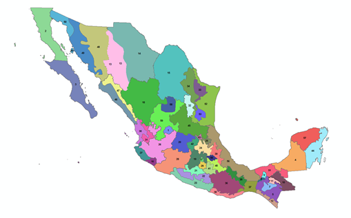
Figure 2 59 regions defined considering coefficients of variation and topographical and meteorological conditions.
Table 3 Number of stations and extreme coefficients of variation in each region
| State | Region | Num. of stations | Maximum Coefficient of Variation | Minimum Coefficient of Variation |
|---|---|---|---|---|
| Aguascalientes | Aguascalientes | 50 | 0.46 | 0.24 |
| Baja California Norte | Baja California Norte | 37 | 1.31 | 0.41 |
| Baja California Sur | Baja California Sur | 72 | 1.36 | 0.46 |
| Campeche | Campeche | 42 | 0.93 | 0.26 |
| Chiapas | Angostura | 36 | 0.88 | 0.22 |
| Malpaso | 17 | 0.66 | 0.24 | |
| Chicoasén | 21 | 0.79 | 0.22 | |
| Peñitas | 4 | 0.51 | 0.26 | |
| Almandro | 11 | 0.82 | 0.24 | |
| Pichucalco | 3 | 0.35 | 0.29 | |
| Teapa | 3 | 0.50 | 0.23 | |
| Costa | 28 | 0.57 | 0.23 | |
| Chihuahua | Bajos | 18 | 0.43 | 0.22 |
| Restantes | 40 | 0.96 | 0.24 | |
| Coahuila | Coahuila | 28 | 1.04 | 0.31 |
| Colima | Colima | 17 | 0.68 | 0.39 |
| Ciudad de México | Ciudad de México | 30 | 0.50 | 0.21 |
| Durango | Durango | 83 | 1.07 | 0.23 |
| Estado de México | Estado de México | 114 | 0.50 | 0.20 |
| Guanajuato | Guanajuato | 108 | 0.49 | 0.22 |
| Guerrero | Norte | 36 | 0.48 | 0.18 |
| Centro | 56 | 0.68 | 0.32 | |
| Costa | 37 | 0.61 | 0.21 | |
| Hidalgo | Menores | 57 | 0.70 | 0.22 |
| Mayores | 5 | 0.52 | 0.43 | |
| Jalisco | Interior | 153 | 0.53 | 0.20 |
| Costa | 23 | 0.58 | 0.30 | |
| Michoacán | Michoacán | 93 | 0.65 | 0.18 |
| Morelos | Morelos | 44 | 0.64 | 0.20 |
| Nayarit | Costa | 14 | 0.40 | 0.25 |
| Sierra | 11 | 0.33 | 0.19 | |
| Nuevo León | I | 10 | 0.93 | 0.29 |
| II | 7 | 0.63 | 0.39 | |
| III | 38 | 1.01 | 0.38 | |
| Oaxaca | Golfo | 29 | 0.53 | 0.26 |
| Altiplano | 82 | 0.74 | 0.18 | |
| Istmo | 14 | 0.56 | 0.37 | |
| Pacifico | 4 | 0.59 | 0.43 | |
| Puebla | Norte | 49 | 0.79 | 0.26 |
| Centro | 34 | 0.67 | 0.21 | |
| Sur | 14 | 0.52 | 0.19 | |
| Querétaro | Zona Alta | 7 | 0.49 | 0.26 |
| Zona Baja | 27 | 0.64 | 0.24 | |
| Quintana Roo | Quintana Roo | 20 | 0.64 | 0.28 |
| San Luis Potosí | San Luis Potosí | 103 | 0.94 | 0.27 |
| Sinaloa | Zona I | 21 | 0.77 | 0.39 |
| Zona II | 30 | 0.62 | 0.20 | |
| Sonora | Zona I | 57 | 0.85 | 0.17 |
| Zona II | 21 | 0.77 | 0.33 | |
| Zona III | 2 | 0.77 | 0.77 | |
| Tabasco | Tabasco | 32 | 0.53 | 0.24 |
| Tamaulipas | Zona I | 81 | 0.87 | 0.27 |
| Zona II | 20 | 0.91 | 0.35 | |
| Zona III | 8 | 0.51 | 0.31 | |
| Tlaxcala | Tlaxcala | 22 | 0.44 | 0.22 |
| Veracruz | Veracruz | 190 | 0.79 | 0.20 |
| Yucatán | Yucatán | 30 | 0.68 | 0.30 |
| Zacatecas | Zona I | 11 | 0.54 | 0.28 |
| Zona II | 39 | 0.45 | 0.22 | |
| Total | 2293 |
Functions of distribution of the regional samples
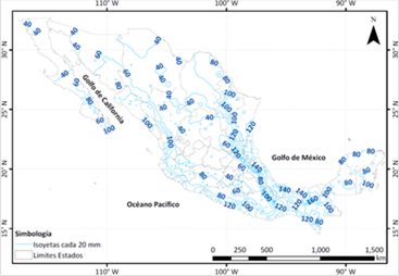
The annual maximum precipitation values of each station were modulated by dividing them into their mean, so that, when grouped together, samples were obtained with considerable number of elements for each of the 59 regions. For each of the 59 extended samples, Gumbel (G) and Double Gumbel (DG) probability distribution functions were fitted, which gave the lowest standard error of fit; the values associated with different return periods were estimated with them as shown as example in Figure 3. Table 4 shows the results obtained for the 59 regions with the probability distributions best fitted. In addition, the average annual precipitation value can be obtained for any site in the Republic, with a map of the distribution of annual maximum precipitation averages (as in Figure 4) and multiplying by the factors by return period corresponding to the region in which the study site is located, to estimate the daily precipitation associated with any return period.
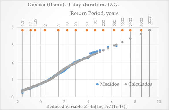
Table 4 Factors per return period for the 59 regions
| State | Homogeneous region | Region | Regionalization factors | |||||||||||
|---|---|---|---|---|---|---|---|---|---|---|---|---|---|---|
| Return Period YEARS | ||||||||||||||
| 2 | 5 | 10 | 20 | 50 | 100 | 200 | 500 | 1 000 | 2 000 | 5 000 | 10 000 | |||
| Aguascalientes | 1 | Aguascalientes | 0.94 | 1.25 | 1.45 | 1.64 | 1.90 | 2.08 | 2.27 | 2.52 | 2.71 | 2.89 | 3.14 | 3.33 |
| 2 | Baja California Norte | 0.84 | 1.36 | 1.81 | 2.23 | 2.73 | 3.09 | 3.45 | 3.91 | 4.27 | 4.62 | 5.09 | 5.43 | |
| Baja California S | 3 | Baja California Sur | 0.77 | 1.36 | 2.03 | 2.65 | 3.38 | 3.90 | 4.41 | 5.08 | 5.57 | 6.07 | 6.72 | 7.21 |
| Campeche | 4 | Campeche | 0.86 | 1.24 | 1.64 | 2.04 | 2.51 | 2.85 | 3.19 | 3.62 | 3.95 | 4.27 | 4.69 | 5.01 |
| Chiapas | 5 | Angostura | 0.90 | 1.19 | 1.46 | 1.81 | 2.29 | 2.65 | 3.00 | 3.46 | 3.81 | 4.15 | 4.61 | 4.95 |
| 6 | Malpaso | 0.90 | 1.22 | 1.50 | 1.80 | 2.20 | 2.49 | 2.77 | 3.15 | 3.44 | 3.72 | 4.10 | 4.36 | |
| 7 | Chicoasén | 0.93 | 1.21 | 1.44 | 1.68 | 1.99 | 2.22 | 2.46 | 2.76 | 2.99 | 3.23 | 3.53 | 3.76 | |
| 8 | Peñitas | 0.91 | 1.22 | 1.50 | 1.79 | 2.18 | 2.47 | 2.76 | 3.13 | 3.41 | 3.69 | 4.07 | 4.35 | |
| 9 | Almandro | 0.89 | 1.22 | 1.53 | 1.89 | 2.36 | 2.70 | 3.03 | 3.47 | 3.80 | 4.13 | 4.55 | 4.90 | |
| 10 | Pichucalco | 0.95 | 1.24 | 1.44 | 1.63 | 1.87 | 2.05 | 2.23 | 2.47 | 2.66 | 2.84 | 3.08 | 3.26 | |
| 11 | Teapa | 0.94 | 1.25 | 1.46 | 1.66 | 1.91 | 2.10 | 2.29 | 2.54 | 2.73 | 2.92 | 3.17 | 3.36 | |
| 12 | Costa | 0.91 | 1.20 | 1.48 | 1.81 | 2.19 | 2.46 | 2.72 | 3.05 | 3.30 | 3.55 | 3.88 | 4.13 | |
| Chihuahua | 13 | Bajos | 0.90 | 1.43 | 1.78 | 2.11 | 2.54 | 2.87 | 3.19 | 3.62 | 3.94 | 4.26 | 4.69 | 5.01 |
| 14 | Restantes | 0.89 | 1.25 | 1.56 | 1.89 | 2.34 | 2.68 | 3.02 | 3.46 | 3.79 | 4.12 | 4.55 | 4.87 | |
| Coahuila | 15 | Coahuila | 0.85 | 1.28 | 1.68 | 2.09 | 2.60 | 2.98 | 3.34 | 3.82 | 4.19 | 4.55 | 5.03 | 5.41 |
| Colima | 16 | Colima | 0.85 | 1.26 | 1.69 | 2.10 | 2.58 | 2.93 | 3.27 | 3.71 | 4.05 | 4.38 | 4.82 | 5.15 |
| Ciudad de México | 17 | Ciudad de México | 0.95 | 1.21 | 1.39 | 1.55 | 1.77 | 1.93 | 2.09 | 2.30 | 2.46 | 2.62 | 2.83 | 3.00 |
| Durango | 18 | Durango | 0.91 | 1.25 | 1.52 | 1.80 | 2.16 | 2.43 | 2.70 | 3.05 | 3.32 | 3.58 | 3.93 | 4.21 |
| Estado de México | 19 | Estado de México | 0.95 | 1.21 | 1.38 | 1.55 | 1.76 | 1.93 | 2.09 | 2.30 | 2.46 | 2.62 | 2.83 | 2.99 |
| Guanajuato | 20 | Guanajuato | 0.95 | 1.23 | 1.42 | 1.60 | 1.83 | 2.00 | 2.17 | 2.40 | 2.57 | 2.75 | 2.98 | 3.15 |
| Guerrero | 21 | Norte | 0.95 | 1.21 | 1.38 | 1.54 | 1.75 | 1.91 | 2.07 | 2.27 | 2.43 | 2.59 | 2.79 | 2.95 |
| 22 | Centro | 0.92 | 1.34 | 1.62 | 1.89 | 2.24 | 2.50 | 2.76 | 3.10 | 3.36 | 3.62 | 3.96 | 4.21 | |
| 23 | Costa | 0.90 | 1.24 | 1.52 | 1.80 | 2.15 | 2.40 | 2.65 | 2.99 | 3.24 | 3.49 | 3.82 | 4.07 | |
| Hidalgo | 24 | Menores | 0.92 | 1.35 | 1.63 | 1.90 | 2.25 | 2.51 | 2.78 | 3.12 | 3.38 | 3.64 | 3.99 | 4.25 |
| 25 | Mayores | 0.87 | 1.35 | 1.71 | 1.98 | 2.30 | 2.53 | 2.76 | 3.06 | 3.28 | 3.50 | 3.80 | 4.01 | |
| Jalisco | 26 | Interior | 0.92 | 1.24 | 1.45 | 1.64 | 1.86 | 2.03 | 2.19 | 2.41 | 2.57 | 2.74 | 2.95 | 3.12 |
| 27 | Costa | 0.93 | 1.30 | 1.55 | 1.79 | 2.09 | 2.32 | 2.55 | 2.85 | 3.08 | 3.31 | 3.61 | 3.84 | |
| Michoacán | 28 | Michoacán | 0.92 | 1.21 | 1.45 | 1.69 | 1.98 | 2.20 | 2.42 | 2.70 | 2.92 | 3.14 | 3.42 | 3.64 |
| Morelos | 29 | Morelos | 0.95 | 1.21 | 1.39 | 1.56 | 1.77 | 1.93 | 2.10 | 2.31 | 2.47 | 2.63 | 2.84 | 3.01 |
| Nayarit | 30 | Costa | 0.95 | 1.22 | 1.40 | 1.58 | 1.80 | 1.97 | 2.13 | 2.36 | 2.52 | 2.69 | 2.91 | 3.08 |
| 31 | Sierra | 0.95 | 1.20 | 1.37 | 1.53 | 1.73 | 1.88 | 2.04 | 2.24 | 2.39 | 2.54 | 2.74 | 2.90 | |
| Nuevo León | 32 | I | 0.88 | 1.26 | 1.61 | 1.99 | 2.51 | 2.89 | 3.26 | 3.75 | 4.12 | 4.49 | 4.97 | 5.34 |
| 33 | II | 0.91 | 1.38 | 1.69 | 1.99 | 2.38 | 2.67 | 2.96 | 3.34 | 3.63 | 3.92 | 4.30 | 4.59 | |
| 34 | III | 0.82 | 1.28 | 1.77 | 2.30 | 2.94 | 3.40 | 3.85 | 4.44 | 4.89 | 5.33 | 5.91 | 6.37 | |
| Oaxaca | 35 | Golfo | 0.94 | 1.24 | 1.44 | 1.63 | 1.87 | 2.06 | 2.24 | 2.48 | 2.66 | 2.84 | 3.08 | 3.27 |
| 36 | Altiplano | 0.91 | 1.22 | 1.46 | 1.76 | 2.2 | 2.53 | 2.86 | 3.28 | 3.6 | 3.92 | 4.33 | 4.64 | |
| 37 | Istmo | 0.87 | 1.36 | 1.72 | 1.97 | 2.27 | 2.48 | 2.69 | 2.96 | 3.17 | 3.38 | 3.65 | 3.85 | |
| 38 | Pacífico | 0.86 | 1.25 | 1.67 | 2.10 | 2.61 | 2.98 | 3.33 | 3.80 | 4.15 | 4.50 | 4.96 | 5.33 | |
| Puebla | 39 | Norte | 0.93 | 1.32 | 1.57 | 1.82 | 2.14 | 2.38 | 2.61 | 2.93 | 3.16 | 3.40 | 3.72 | 3.95 |
| 40 | Centro | 0.94 | 1.27 | 1.49 | 1.71 | 1.98 | 2.19 | 2.40 | 2.67 | 2.87 | 3.08 | 3.35 | 3.55 | |
| 41 | Sur | 0.94 | 1.26 | 1.47 | 1.67 | 1.92 | 2.12 | 2.31 | 2.57 | 2.76 | 2.95 | 3.21 | 3.40 | |
| Querétaro | 42 | Zona Alta | 0.93 | 1.29 | 1.53 | 1.75 | 2.04 | 2.26 | 2.48 | 2.77 | 2.99 | 3.21 | 3.49 | 3.71 |
| 43 | Zona Baja | 0.94 | 1.27 | 1.49 | 1.70 | 1.98 | 2.18 | 2.38 | 2.65 | 2.86 | 3.06 | 3.33 | 3.53 | |
| Quintana Roo | 44 | Quintana Roo | 0.88 | 1.26 | 1.60 | 1.91 | 2.28 | 2.55 | 2.82 | 3.17 | 3.44 | 3.70 | 4.05 | 4.32 |
| San Luis | 45 | San Luis | 0.88 | 1.29 | 1.63 | 1.94 | 2.33 | 2.61 | 2.89 | 3.25 | 3.52 | 3.80 | 4.16 | 4.44 |
| Sinaloa | 46 | Zona I | 0.84 | 1.28 | 1.76 | 2.15 | 2.61 | 2.93 | 3.25 | 3.67 | 3.98 | 4.29 | 4.70 | 5.01 |
| 47 | Zona II | 0.94 | 1.27 | 1.49 | 1.70 | 1.97 | 2.18 | 2.38 | 2.65 | 2.85 | 3.06 | 3.33 | 3.53 | |
| Sonora | 48 | Zona I | 0.93 | 1.29 | 1.53 | 1.75 | 2.05 | 2.27 | 2.49 | 2.78 | 3.00 | 3.22 | 3.50 | 3.72 |
| 49 | Zona II | 0.88 | 1.26 | 1.61 | 1.96 | 2.38 | 2.69 | 3.00 | 3.40 | 3.70 | 4.00 | 4.41 | 4.71 | |
| 50 | Zona III | 0.77 | 1.50 | 2.23 | 2.77 | 3.38 | 3.82 | 4.25 | 4.82 | 5.24 | 5.67 | 6.22 | 6.64 | |
| Tabasco | 51 | Tabasco | 0.94 | 1.26 | 1.47 | 1.67 | 1.94 | 2.13 | 2.33 | 2.59 | 2.78 | 2.98 | 3.23 | 3.43 |
| Tamaulipas | 52 | Zona I | 0.89 | 1.31 | 1.61 | 1.88 | 2.20 | 2.43 | 2.66 | 2.96 | 3.19 | 3.42 | 3.72 | 3.95 |
| 53 | Zona II | 0.85 | 1.26 | 1.69 | 2.18 | 2.81 | 3.26 | 3.70 | 4.27 | 4.71 | 5.14 | 5.72 | 6.12 | |
| 54 | Zona III | 0.91 | 1.32 | 1.59 | 1.82 | 2.09 | 2.29 | 2.49 | 2.75 | 2.94 | 3.14 | 3.39 | 3.59 | |
| Tlaxcala | 55 | Tlaxcala | 0.95 | 1.22 | 1.40 | 1.57 | 1.79 | 1.96 | 2.13 | 2.35 | 2.51 | 2.68 | 2.90 | 3.06 |
| Veracruz | 56 | Veracruz | 0.90 | 1.27 | 1.56 | 1.83 | 2.15 | 2.39 | 2.62 | 2.93 | 3.16 | 3.39 | 3.69 | 3.93 |
| Yucatán | 57 | Yucatán | 0.93 | 1.32 | 1.59 | 1.84 | 2.17 | 2.41 | 2.66 | 2.98 | 3.22 | 3.47 | 3.79 | 4.03 |
| Zacatecas | 58 | Zona I | 0.92 | 1.34 | 1.62 | 1.88 | 2.23 | 2.48 | 2.74 | 3.08 | 3.33 | 3.59 | 3.92 | 4.18 |
| 59 | Zona II | 0.95 | 1.23 | 1.42 | 1.60 | 1.84 | 2.02 | 2.19 | 2.42 | 2.60 | 2.77 | 3.00 | 3.18 | |
Estimates for storms with durations less than 1h
Figure 5 shows the map of convectivity factors estimated by Baeza (2007). To obtain the precipitation associated with a duration of 1h, only multiply that obtained for one day by the corresponding factor. In addition, and according to the results obtained by Chen (1983), to estimate the values associated with other durations of less than 24 h, those of 1 h are multiplied by the factors indicated in Table 5.
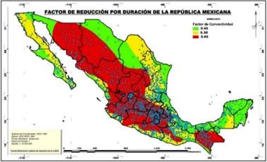
Table 5 Factors K d (1) depending on R to and duration d. Source: Adapted from Luna, 2013
| d(min) | d(hrs) |
|
|||||||
|---|---|---|---|---|---|---|---|---|---|
| R=0.10 | R=0.20 | R=0.30 | R=0.40 | R=0.45 | R=0.50 | R=0.60 | R=0.65 | ||
| 10 | 0.17 | 0.293 | 0.39 | 0.432 | 0.454 | 0.462 | 0.469 | 0.481 | 0.487 |
| 15 | 0.25 | 0.38 | 0.485 | 0.536 | 0.565 | 0.575 | 0.584 | 0.6 | 0.608 |
| 30 | 0.5 | 0.612 | 0.699 | 0.745 | 0.773 | 0.79 | 0.793 | 0.809 | 0.816 |
| 60 | 1 | 1 | 1 | 1 | 1 | 1 | 1 | 1 | 1 |
| 90 | 1.5 | 1.378 | 1.248 | 1.185 | 1.146 | 1.13 | 1.119 | 1.097 | 1.088 |
| 120 | 2 | 1.646 | 1.424 | 1.317 | 1.25 | 1.22 | 1.203 | 1.166 | 1.151 |
| 150 | 2.5 | 1.934 | 1.595 | 1.435 | 1.337 | 1.30 | 1.268 | 1.215 | 1.193 |
| 180 | 3 | 2.207 | 1.75 | 1.538 | 1.41 | 1.35 | 1.322 | 1.254 | 1.226 |
| 210 | 3.5 | 2.468 | 1.892 | 1.631 | 1.475 | 1.41 | 1.367 | 1.286 | 1.253 |
| 240 | 4 | 2.719 | 2.024 | 1.715 | 1.532 | 1.45 | 1.407 | 1.314 | 1.275 |
| 270 | 4.5 | 2.961 | 2.148 | 1.793 | 1.584 | 1.508 | 1.443 | 1.337 | 1.294 |
| 300 | 5 | 3.196 | 2.266 | 1.865 | 1.631 | 1.547 | 1.475 | 1.358 | 1.311 |
| 360 | 6 | 3.649 | 2.485 | 1.997 | 1.716 | 1.616 | 1.531 | 1.395 | 1.339 |
| 420 | 7 | 4.081 | 2.686 | 2.115 | 1.791 | 1.676 | 1.579 | 1.425 | 1.362 |
| 480 | 8 | 4.497 | 2.874 | 2.223 | 1.858 | 1.73 | 1.621 | 1.451 | 1.382 |
| 540 | 9 | 4.899 | 3.05 | 2.322 | 1.919 | 1.778 | 1.659 | 1.474 | 1.399 |
| 600 | 10 | 5.289 | 3.216 | 2.414 | 1.975 | 1.822 | 1.694 | 1.494 | 1.415 |
| 660 | 11 | 5.669 | 3.375 | 2.501 | 2.026 | 1.862 | 1.725 | 1.513 | 1.429 |
| 720 | 12 | 6.039 | 3.527 | 2.582 | 2.074 | 1.9 | 1.754 | 1.53 | 1.441 |
| 840 | 14 | 6.756 | 3.812 | 2.734 | 2.162 | 1.968 | 1.807 | 1.56 | 1.463 |
| 960 | 16 | 7.445 | 4.078 | 2.872 | 2.241 | 2.029 | 1.853 | 1.586 | 1.482 |
| 1080 | 18 | 8.112 | 4.328 | 2.999 | 2.313 | 2.084 | 1.895 | 1.609 | 1.499 |
| 1200 | 20 | 8.758 | 4.564 | 3.117 | 2.379 | 2.134 | 1.933 | 1.63 | 1.513 |
| 1320 | 22 | 9.388 | 4.789 | 3.228 | 2.441 | 2.18 | 1.968 | 1.649 | 1.527 |
| 1440 | 24 | 10.001 | 5.004 | 3.333 | 2.498 | 2.223 | 2 | 1.667 | 1.539 |
Estimates for durations greater than one day
When studies are conducted for large basins or inputs to dams with significant regulatory capacity, it is required to have multi-day design storms. For this reason, the analysis of the historical data of the average maximum annual precipitations associated with durations of 2, 3,..., 30 consecutive days was performed. For each station i and each year of registration k the ratio was obtained between the average maximum rainfall corresponding to each duration and the corresponding to one day, that is:
where PMAXd,i,k is the maximum average rainfall for a duration d, in days, in a station i and year k.
When making the averages for all the record years of the station i, it is obtained:
Where NK are the record years.
Then, for each region, the averages were obtained by considering all stations:
Where NI is the number of stations in the region considered
Table 6 shows the values obtained for each region and durations of 2 and 8 days; it is noted the small difference between the values obtained for the different regions, so that, for example, for the duration of 2 days, 75% of the values are between 0.66 and 0.702 and for 8 days, more than 80% are between 0.26 and 0.34. In summary, the results obtained in this study allow to obtain, for any site of the Republic, values of average precipitation associated to different return periods, for durations between 15 minutes and 30 days.
Table 6 Relationship between maximum average rainfall associated with different durations and those corresponding to one day
| REGION | NUMBER OF VALUES | 2D/1D | 8D/1D | REGION | NUMBER OF VALUES | 2D/1D | 8D/1D |
|---|---|---|---|---|---|---|---|
| Chiapas, Pichucalco | 3 | 0.686 | 0.32 | HGOMEN | 58 | 0.667 | 0.287 |
| Chiapas, Chicoasén | 20 | 0.677 | 0.325 | JALCOST | 23 | 0.669 | 0.291 |
| Chiapas, Almandro | 11 | 0.693 | 0.332 | JALINT | 153 | 0.67 | 0.309 |
| Chiapas, Teapa | 3 | 0.69 | 0.313 | MIH000 | 93 | 0.668 | 0.324 |
| Chiapas, Malpaso | 17 | 0.668 | 0.298 | OAXALT | 82 | 0.693 | 0.33 |
| Chiapas, Angostura | 36 | 0.697 | 0.341 | OAXGOL | 29 | 0.693 | 0.338 |
| Peñitas | 4 | 0.69 | 0.299 | OAXPAC | 4 | 0.667 | 0.319 |
| Chiapas Costa | 28 | 0.687 | 0.329 | OAXITS | 14 | 0.687 | 0.282 |
| Tlaxcala | 22 | 0.673 | 0.314 | PUECEN | 34 | 0.687 | 0.32 |
| Yucatán | 32 | 0.64 | 0.258 | PUENOR | 49 | 0.699 | 0.314 |
| Morelos | 44 | 0.681 | 0.331 | PUESUR | 14 | 0.664 | 0.311 |
| Zacatecas, Zona 01 | 11 | 0.664 | 0.272 | Querétaro, ZonaBaja | 26 | 0.666 | 0.281 |
| Zacatecas, Zona 02 | 39 | 0.67 | 0.295 | Querétaro, Zona Alta | 7 | 0.702 | 0.319 |
| Nuevo León, Región 1 | 9 | 0.66 | 0.259 | Sinaloa,Zona I | 21 | 0.599 | 0.212 |
| Nuevo León, Región 2 | 7 | 0.623 | 0.223 | Sinaloa, Zona II | 30 | 0.622 | 0.247 |
| Nuevo León, Región 3 | 38 | 0.656 | 0.242 | SLP000 | 103 | 0.682 | 0.289 |
| Ciudad de México | 34 | 0.675 | 0.323 | SONRE1 | 57 | 0.62 | 0.238 |
| Colima | 17 | 0.669 | 0.26 | SONRE2 | 21 | 0.583 | 0.199 |
| Guanajuato | 106 | 0.678 | 0.31 | SONRE3 | 2 | 0.585 | 0.169 |
| Veracruz | 182 | 0.687 | 0.304 | TAMZ01 | 81 | 0.664 | 0.266 |
| Chihuahua,restantes | 40 | 0.646 | 0.26 | TAMZ02 | 20 | 0.662 | 0.266 |
| CHIBAJ | 18 | 0.669 | 0.294 | TAMZ03 | 8 | 0.654 | 0.265 |
| AGS000 | 50 | 0.684 | 0.298 | CAM000 | 44 | 0.658 | 0.283 |
| COA000 | 34 | 0.628 | 0.219 | DUR000 | 83 | 0.677 | 0.29 |
| EDM000 | 114 | 0.673 | 0.329 | TAB000 | 32 | 0.668 | 0.278 |
| GUECEN | 55 | 0.689 | 0.309 | Nayarit, Costa | 14 | 0.634 | 0.282 |
| GUECOS | 38 | 0.69 | 0.335 | Nayarit, Sierra | 11 | 0.682 | 0.322 |
| GUENOR | 36 | 0.669 | 0.321 | BCN000 | 38 | 0.644 | 0.222 |
| HGOMAY | 8 | 0.708 | 0.313 | BCS000 | 75 | 0.61 | 0.187 |
Example for interpretation of results
To facilitate the interpretation of the results obtained, the following example is proposed:
Suppose that the centroid of a basin in the Oaxaca Istmo region has coordinates -94,559 Longitude West and 16.733 Latitude North, in such a way that the average of the maximum annual daily precipitation is 140 mm (see Figure 4, or for more detail Figure 6). According to Table 4, this value is multiplied by 2.48 to estimate the precipitation associated with 100 years of return period, resulting in a value of 347.2 mm for 1-day rainfall with 100 years of return period. If the concentration-time of the watershed was 1.5 h, a hyetograph with half-hour intervals and a total duration of 4 h could be estimated as follows. According to Figure 7, the convectivity factor would be 0.45, so that the precipitation in 1 h results in 156.2 mm. For this value of the convectivity factor, Table 5 indicates the factors to be considered for the different durations. These factors are reproduced in Table 7. The third column of Table 7 was obtained by multiplying the factors by 156.2 mm; in the fourth one the increments are indicated every half hour and in the fifth those same values ordered by alternate blocks, to obtain the hyetograph of Figure 7.
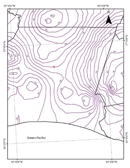
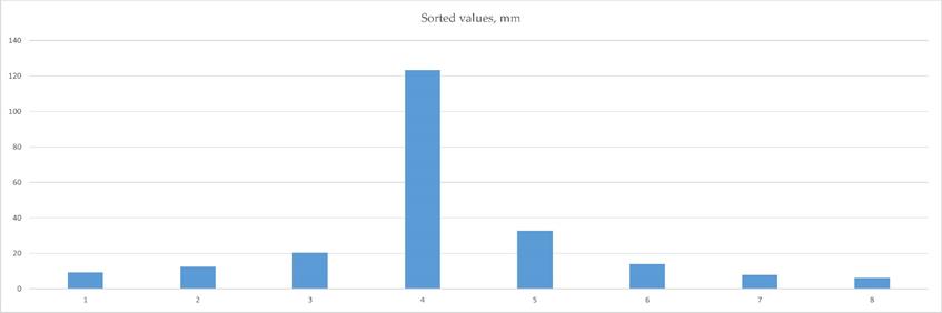
Table 7 Estimation of a hyetograph for 30-minute intervals and total duration of 4 h
| Duration minutes | Factor respect to 1h | Accumulated precipitation (mm) | Increment (mm) | Sorted values (mm) |
|---|---|---|---|---|
| 30 | 0.79 | 148.52 | 148.52 | 10.68 |
| 60 | 1.00 | 188.00 | 39.48 | 14.80 |
| 90 | 1.13 | 213.31 | 25.31 | 25.31 |
| 120 | 1.22 | 229.36 | 16.05 | 148.52 |
| 150 | 1.30 | 244.16 | 14.80 | 39.48 |
| 180 | 1.35 | 253.80 | 9.64 | 16.05 |
| 210 | 1.41 | 264.48 | 10.68 | 9.64 |
| 240 | 1.45 | 272.60 | 8.12 | 8.12 |
Discussion
The results obtained allow to estimate in a robust and spatially consistent manner, rainfall for any part of the republic, any period of return and any duration. With these results, design hyetographs can also be built.
To verify the statistically homogeneous behavior of the maximum rainfall sample data in a region, the Fisher test is used traditionally, comparing the ratios of the variances corresponding to the different sites to the limits of the Fisher distribution function for a probability of being exceeded by, for example, 5%.
The values obtained from the squared ratios of the coefficients of maximum variation between the minimum of each region are shown in Table 8, which also indicates the type of distribution function that best fit the extended sample corresponding to each region.
Table 8 Relations between the coefficients of maximum and minimum variation of the stations included in each region
| State | Region | Number Stations | Coef. var. MAXIMUM | Coef. var. MINIMUM | Squared ratio | Distribution Function* |
|---|---|---|---|---|---|---|
| Aguascalientes | Aguascalientes | 50 | 0.46 | 0.24 | 3.67 | G |
| Baja California Norte | Baja California Norte | 37 | 1.31 | 0.41 | 10.21 | DG |
| Baja California Sur | Baja California Sur | 72 | 1.36 | 0.46 | 8.74 | DG |
| Campeche | Campeche | 42 | 0.93 | 0.26 | 12.79 | DG |
| Chiapas | Angostura | 36 | 0.88 | 0.22 | 16.00 | DG |
| Malpaso | 17 | 0.66 | 0.24 | 7.56 | DG | |
| Chicoasén | 21 | 0.79 | 0.22 | 12.89 | DG | |
| Peñitas | 4 | 0.51 | 0.26 | 3.85 | DG | |
| Almandro | 11 | 0.82 | 0.24 | 11.67 | DG | |
| Pichucalco | 3 | 0.35 | 0.29 | 1.46 | G | |
| Teapa | 3 | 0.50 | 0.23 | 4.73 | G | |
| Costa | 28 | 0.57 | 0.23 | 6.14 | DG | |
| Chihuahua | Bajos | 18 | 0.43 | 0.22 | 3.82 | G |
| Restantes | 40 | 0.96 | 0.24 | 16.00 | DG | |
| Coahuila | Coahuila | 28 | 1.04 | 0.31 | 11.25 | DG |
| Colima | Colima | 17 | 0.68 | 0.39 | 3.04 | DG |
| Distrito Federal | Distrito Federal | 30 | 0.50 | 0.21 | 5.67 | G |
| Durango | Durango | 83 | 1.07 | 0.23 | 21.64 | DG |
| Estado de México | Estado de México | 114 | 0.50 | 0.20 | 6.25 | G |
| Guanajuato | Guanajuato | 108 | 0.49 | 0.22 | 4.96 | G |
| Guerrero | Norte | 36 | 0.48 | 0.18 | 7.11 | G |
| Centro | 56 | 0.68 | 0.32 | 4.52 | G | |
| Costa | 37 | 0.61 | 0.21 | 8.44 | DG | |
| Hidalgo | Menores | 57 | 0.70 | 0.22 | 10.12 | G |
| Mayores | 5 | 0.52 | 0.43 | 1.46 | G | |
| Jalisco | Interior | 153 | 0.53 | 0.20 | 7.02 | G |
| Costa | 23 | 0.58 | 0.30 | 3.74 | G | |
| Michoacán | Michoacán | 93 | 0.65 | 0.18 | 13.04 | G |
| Morelos | Morelos | 44 | 0.64 | 0.20 | 10.24 | G |
| Nayarit | Costa | 14 | 0.40 | 0.25 | 2.56 | G |
| Sierra | 11 | 0.33 | 0.19 | 3.02 | G | |
| Nuevo León | I | 10 | 0.93 | 0.29 | 10.28 | DG |
| II | 7 | 0.63 | 0.39 | 2.61 | DG | |
| III | 38 | 1.01 | 0.38 | 7.06 | DG | |
| Oaxaca | Golfo | 29 | 0.53 | 0.26 | 4.16 | G |
| Altiplano | 82 | 0.74 | 0.18 | 16.90 | DG | |
| Istmo | 14 | 0.56 | 0.37 | 2.29 | DG | |
| Pacífico | 4 | 0.59 | 0.43 | 1.88 | DG | |
| Puebla | Norte | 49 | 0.79 | 0.26 | 9.23 | G |
| Centro | 34 | 0.67 | 0.21 | 10.18 | G | |
| Sur | 14 | 0.52 | 0.19 | 7.49 | G | |
| Querétaro | Zona Alta | 7 | 0.49 | 0.26 | 3.55 | G |
| Zona Baja | 27 | 0.64 | 0.24 | 7.11 | G | |
| Quintana Roo | Quintana Roo | 20 | 0.64 | 0.28 | 5.22 | DG |
| San Luis | San Luis | 103 | 0.94 | 0.27 | 12.12 | DG |
| Sinaloa | Zona I | 21 | 0.77 | 0.39 | 3.90 | DG |
| Zona II | 30 | 0.62 | 0.20 | 9.61 | G | |
| Sonora | Zona I | 57 | 0.85 | 0.17 | 23.90 | G |
| Zona II | 21 | 0.77 | 0.33 | 5.44 | DG | |
| Zona III | 2 | 0.77 | 0.77 | 1.00 | DG | |
| Tabasco | Tabasco | 32 | 0.53 | 0.24 | 4.88 | G |
| Tamaulipas | Zona I | 81 | 0.87 | 0.27 | 10.38 | DG |
| Zona II | 20 | 0.91 | 0.35 | 6.76 | DG | |
| Zona III | 8 | 0.51 | 0.31 | 2.71 | DG | |
| Tlaxcala | Tlaxcala | 22 | 0.44 | 0.22 | 4.00 | G |
| Veracruz | Veracruz | 190 | 0.79 | 0.20 | 15.60 | DG |
| Yucatán | Yucatán | 30 | 0.68 | 0.30 | 5.13 | G |
| Zacatecas | Zona I | 11 | 0.54 | 0.28 | 3.72 | G |
| Zona II | 39 | 0.45 | 0.22 | 4.18 | G | |
| Total | 2293 |
*G: Gumbel DG: Double Gumbel
The analysis in Table 8 shows that, in some cases, the square of the ratio between the maximum and minimum coefficients of variation is very large, so that in applying the Fisher test, it would be concluded that some stations should be removed from the corresponding region, although care was taken to ensure that climates and exposure to similar meteorological phenomena were present for each region and that the separation between regions corresponded to a well-defined watershed. It is also noted in Table 8 that most of these cases correspond to regions in which the best fit for the enlarged sample was obtained with the Double Gumbel Function. Two very notable cases are Sonora zone 1 and Veracruz, so these two cases are commented next: in Sonora, the largest CV (0.85) was in station 26034, in which, in 1972, a maximum of 407 mm was recorded whereas, of all the other stations the maximum measured was of 176 mm, and in all the period of record of all the stations the maximum measured is of 240 mm; if it is eliminated, the CV of the maximums in that station would be of 0.525.At the other extreme, the minimum CV value is 0.174 and corresponds to station 26101 in which the maximum recorded is very low (106 mm) even though the average is one of the highest in the region, possibly because it did not record in the years in which the major storms occurred (1978, 1994 and 2007). If these two values are eliminated, the extreme CV are left at 0.69 (at station 26010 which did measure in critical years) and 0.211, so that the squared ratio is 10.6 instead of 23.9; if the two extreme values are still eliminated, the squared ratio is 3.89.
Something similar occurs in Veracruz, where there is a record of 690 mm in the station 30031, in 1978, a year that was not characterized by major storms and in which the maximum recorded in the other 189 stations was 364 mm. If that value is eliminated, the maximum CV results from 0.67 and the square ratio between extreme values is reduced from 15.60 to 11.2. Also, if the two smaller values of the CV are eliminated from the 190 stations in this region, the ratio is reduced to 7.2, a value which is logical if it is considered to correspond to 187 stations.
Generation of synthetic series
Considering that these are extreme events whose probability distribution is not Normal, tests were performed by comparing the coefficients of variation of the historical samples to those obtained by generating random numbers with the adjusted probability distribution to the regional samples. For each of the 59 regions, 10 synthetic samples were generated, with the same number of values as the corresponding historical sample. Figures 8 and 9 compare the cumulative frequency distributions of the historical and synthetic CV for the extreme cases of the regions in Morelos and La Angostura in Chiapas. In each case 10 synthetic samples were generated, each of which consists of the same number of values as the one of years recorded in each station of the corresponding region.
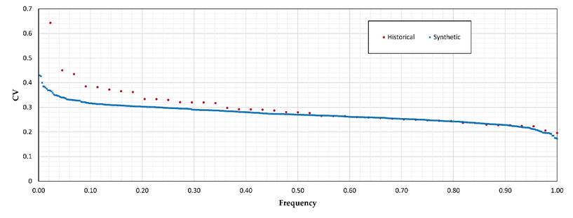
Figure 8 Comparison between the empirical frequencies of the coefficients of variation of the historical sample and the sample generated. Morelos Region
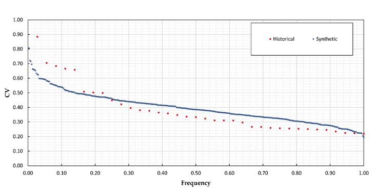
Figure 9 Comparison between the empirical frequencies of the coefficients of variation of the historical sample and the sample generated. La Angostura Region, in Chiapas
In the first case (Morelos region) a good behavior is observed except for a station with a coefficient of variation of 0.64, (which was the maximum in that area in which the next value was 0.45). The station is number 17045 and in its data of maximum annual precipitations appears a value of 200 mm in 1977, year in which the maximum registered in all the other stations was of 87 mm, reason why it was resorted to verify the data, with the help of GASIR, in the original registry, and it was found that the maximum in that year was 57.4 and when changing it the coefficient of variation fell to 0.332.
In the case of the Angostura region, in Chiapas, although the behavior of the relative frequencies of the historical CV and the CV generated is similar (Figure 9) the value of the historical maximum CV (0.88, corresponding to station 7119, with 66 years ) was higher than the maximum generated with the 10 synthetic samples (0.81), so it was analyzed in more detail and was found to correspond to a record of 320 mm on October 5, 2005, when several high values were presented in the near stations, reason why it was decided to conserve that value.
Table 9 shows the coefficients of variation of each of the other 12 regions (of the 59 considered) in which the square ratio of the coefficients of variation is greater than 10.
Table 9 Variation coefficients of each station for the 12 regions (out of the 59 considered) in which the square ratio of the coefficients of variation is greater than 10.
| BCN | Campeche | Chiapas | Chiapas | Chihuahua | Coahuila | Durango | Hidalgo | Michoacán | Oaxaca | Puebla | Nuevo León |
|---|---|---|---|---|---|---|---|---|---|---|---|
| Chicoasén | Almandro | Restantes | Menores | Altiplano | Centro | Reg. 1 | |||||
| Coef. var. | Coef. var. | Coef. var. | Coef. var. | Coef. var. | Coef. var. | Coef. var. | Coef. var. | Coef. var. | Coef. var. | Coef. var. | Coef. var. |
| 1.315 | 0.934 | 0.792 | 0.822 | 0.958 | 1.044 | 1.070 | 0.700 | 0.647 | 0.738 | 0.669 | 0.933 |
| 0.969 | 0.658 | 0.461 | 0.465 | 0.714 | 0.875 | 0.879 | 0.620 | 0.618 | 0.680 | 0.483 | 0.573 |
| 0.950 | 0.655 | 0.409 | 0.410 | 0.662 | 0.744 | 0.634 | 0.602 | 0.593 | 0.662 | 0.481 | 0.522 |
| 0.826 | 0.643 | 0.389 | 0.406 | 0.655 | 0.632 | 0.583 | 0.569 | 0.586 | 0.648 | 0.438 | 0.499 |
| 0.777 | 0.635 | 0.386 | 0.383 | 0.601 | 0.628 | 0.582 | 0.535 | 0.555 | 0.598 | 0.393 | 0.475 |
| 0.776 | 0.634 | 0.367 | 0.369 | 0.599 | 0.624 | 0.561 | 0.516 | 0.501 | 0.588 | 0.386 | 0.433 |
| 0.738 | 0.627 | 0.365 | 0.312 | 0.492 | 0.609 | 0.523 | 0.515 | 0.494 | 0.565 | 0.376 | 0.418 |
| 0.663 | 0.596 | 0.350 | 0.308 | 0.489 | 0.597 | 0.521 | 0.513 | 0.490 | 0.564 | 0.375 | 0.355 |
| 0.616 | 0.594 | 0.330 | 0.298 | 0.484 | 0.596 | 0.513 | 0.512 | 0.449 | 0.557 | 0.371 | 0.322 |
| 0.602 | 0.579 | 0.326 | 0.264 | 0.482 | 0.591 | 0.505 | 0.502 | 0.440 | 0.557 | 0.355 | 0.289 |
| 0.596 | 0.576 | 0.296 | 0.245 | 0.479 | 0.588 | 0.502 | 0.497 | 0.435 | 0.557 | 0.355 | |
| 0.581 | 0.554 | 0.286 | 0.469 | 0.553 | 0.492 | 0.485 | 0.435 | 0.554 | 0.354 | ||
| 0.581 | 0.544 | 0.272 | 0.467 | 0.548 | 0.485 | 0.472 | 0.427 | 0.537 | 0.352 | ||
| 0.572 | 0.540 | 0.272 | 0.457 | 0.529 | 0.484 | 0.464 | 0.425 | 0.532 | 0.332 | ||
| 0.571 | 0.512 | 0.269 | 0.455 | 0.513 | 0.481 | 0.448 | 0.417 | 0.526 | 0.331 | ||
| 0.570 | 0.511 | 0.266 | 0.442 | 0.510 | 0.480 | 0.447 | 0.411 | 0.513 | 0.331 | ||
| 0.570 | 0.511 | 0.246 | 0.437 | 0.497 | 0.477 | 0.444 | 0.409 | 0.505 | 0.324 | ||
| 0.556 | 0.503 | 0.237 | 0.435 | 0.497 | 0.454 | 0.433 | 0.404 | 0.500 | 0.323 | ||
| 0.550 | 0.478 | 0.234 | 0.432 | 0.495 | 0.453 | 0.430 | 0.395 | 0.491 | 0.318 | ||
| 0.550 | 0.473 | 0.219 | 0.429 | 0.491 | 0.452 | 0.428 | 0.394 | 0.477 | 0.308 | ||
| 0.545 | 0.465 | 0.427 | 0.491 | 0.450 | 0.420 | 0.390 | 0.466 | 0.300 | |||
| 0.528 | 0.461 | 0.417 | 0.490 | 0.447 | 0.420 | 0.381 | 0.458 | 0.289 | |||
| 0.528 | 0.461 | 0.412 | 0.490 | 0.440 | 0.408 | 0.376 | 0.432 | 0.287 | |||
| 0.520 | 0.459 | 0.411 | 0.482 | 0.438 | 0.404 | 0.374 | 0.428 | 0.285 | |||
| 0.517 | 0.458 | 0.404 | 0.466 | 0.433 | 0.402 | 0.373 | 0.427 | 0.279 | |||
| 0.516 | 0.454 | 0.399 | 0.462 | 0.432 | 0.400 | 0.368 | 0.418 | 0.272 | |||
| 0.510 | 0.445 | 0.398 | 0.444 | 0.431 | 0.389 | 0.365 | 0.410 | 0.266 | |||
| 0.507 | 0.436 | 0.395 | 0.436 | 0.431 | 0.387 | 0.364 | 0.408 | 0.265 | |||
| 0.482 | 0.436 | 0.364 | 0.435 | 0.429 | 0.387 | 0.361 | 0.406 | 0.263 | |||
| 0.477 | 0.432 | 0.352 | 0.429 | 0.423 | 0.382 | 0.360 | 0.404 | 0.255 | |||
| 0.476 | 0.424 | 0.340 | 0.428 | 0.419 | 0.378 | 0.358 | 0.402 | 0.252 | |||
| 0.469 | 0.419 | 0.335 | 0.404 | 0.415 | 0.362 | 0.357 | 0.401 | 0.244 | |||
| 0.459 | 0.412 | 0.328 | 0.369 | 0.414 | 0.354 | 0.349 | 0.399 | 0.244 | |||
| 0.450 | 0.412 | 0.319 | 0.321 | 0.408 | 0.354 | 0.349 | 0.398 | 0.210 | |||
| 0.440 | 0.394 | 0.317 | 0.313 | 0.406 | 0.351 | 0.348 | 0.390 | ||||
| 0.421 | 0.381 | 0.315 | 0.405 | 0.342 | 0.339 | 0.387 | |||||
| 0.420 | 0.374 | 0.303 | 0.401 | 0.339 | 0.339 | 0.381 | |||||
| 0.407 | 0.367 | 0.279 | 0.399 | 0.334 | 0.338 | 0.380 | |||||
| 0.366 | 0.263 | 0.393 | 0.330 | 0.333 | 0.373 | ||||||
| 0.363 | 0.240 | 0.389 | 0.326 | 0.333 | 0.369 | ||||||
| 0.360 | 0.385 | 0.324 | 0.333 | 0.368 | |||||||
| 0.344 | 0.384 | 0.323 | 0.330 | 0.367 | |||||||
| 0.335 | 0.379 | 0.319 | 0.329 | 0.366 | |||||||
| 0.303 | 0.379 | 0.315 | 0.328 | 0.363 | |||||||
| 0.288 | 0.373 | 0.309 | 0.324 | 0.363 | |||||||
| 0.263 | 0.370 | 0.307 | 0.320 | 0.358 | |||||||
| 0.367 | 0.306 | 0.317 | 0.354 | ||||||||
| 0.366 | 0.297 | 0.315 | 0.354 | ||||||||
| 0.365 | 0.293 | 0.313 | 0.353 | ||||||||
| 0.365 | 0.288 | 0.311 | 0.350 | ||||||||
| 0.362 | 0.285 | 0.310 | 0.348 | ||||||||
| 0.362 | 0.272 | 0.308 | 0.348 | ||||||||
| 0.361 | 0.271 | 0.307 | 0.348 | ||||||||
| 0.357 | 0.265 | 0.305 | 0.344 | ||||||||
| 0.357 | 0.260 | 0.303 | 0.340 | ||||||||
| 0.354 | 0.249 | 0.303 | 0.340 | ||||||||
| 0.354 | 0.229 | 0.301 | 0.340 | ||||||||
| 0.354 | 0.218 | 0.295 | 0.339 | ||||||||
| 0.350 | 0.293 | 0.338 | |||||||||
| 0.349 | 0.292 | 0.315 | |||||||||
| 0.346 | 0.290 | 0.312 | |||||||||
| 0.341 | 0.289 | 0.311 | |||||||||
| 0.339 | 0.288 | 0.309 | |||||||||
| 0.337 | 0.288 | 0.307 | |||||||||
| 0.334 | 0.284 | 0.304 | |||||||||
| 0.329 | 0.283 | 0.297 | |||||||||
| 0.325 | 0.281 | 0.295 | |||||||||
| 0.315 | 0.281 | 0.294 | |||||||||
| 0.299 | 0.280 | 0.287 | |||||||||
| 0.298 | 0.274 | 0.282 | |||||||||
| 0.298 | 0.272 | 0.282 | |||||||||
| 0.282 | 0.272 | 0.276 | |||||||||
| 0.279 | 0.267 | 0.275 | |||||||||
| 0.276 | 0.260 | 0.273 | |||||||||
| 0.275 | 0.257 | 0.272 | |||||||||
| 0.273 | 0.255 | 0.258 | |||||||||
| 0.266 | 0.247 | 0.253 | |||||||||
| 0.266 | 0.246 | 0.251 | |||||||||
| 0.260 | 0.244 | 0.241 | |||||||||
| 0.253 | 0.243 | 0.241 | |||||||||
| 0.251 | 0.241 | 0.202 | |||||||||
| 0.238 | 0.231 | 0.175 | |||||||||
| 0.228 | 0.231 | ||||||||||
| 0.230 | |||||||||||
| 0.229 | |||||||||||
| 0.221 | |||||||||||
| 0.220 | |||||||||||
| 0.208 | |||||||||||
| 0.207 | |||||||||||
| 0.199 | |||||||||||
| 0.198 | |||||||||||
| 0.186 | |||||||||||
| 0.180 |
For each of these 12 regions, 10 synthetic samples were also generated, each with the same number of values as the historical record. In Table 9, the historical coefficients of variation greater than 20% of the maximum obtained with the generated series were marked with green, which are greater or less than the extreme values obtained with the samples generated but in which the differences are less than 20%. It can be observed that of the 12 regions, in five of them the historical coefficient of variation exceeds the synthetic by more than 20% and in one there are two stations in which this occurs; there are also 13 stations (of more than 2000 studied) in which the historical coefficient of variation exceeds the synthetic one but in less than 20%, and eight in which the historical minimum is less than the synthetic one in less than 20%. For the cases that appeared to be the strangest, a request for verification was made to CONAGUA's Superficial Water Management and Engineering (GASIR), with the results shown in Table 10. According to the information provided by GASIR, the values of the coefficients of variation of table 8 are modified as follows:
Table 10 Results of doubtful data verification
| DOUBTFUL DATA ON CLIMATOLOGICAL STATIONS | ||||||
|---|---|---|---|---|---|---|
| State | Station | Value (mm) | Year | Month | Day | |
| Baja California Norte | 2046 | 240 | 1972 | 10 | 4 | GASIR recommends elimination |
| 2046 | 170 | 1973 | 9 | 25 | GASIR does not find information, it was eliminated | |
| Campeche | 4006 | 380 | 1950 | 10 | 8 | GASIR says it is 38 |
| 4006 | 200 | 1995 | 8 | 20 | Correct | |
| Chiapas | 7033 | 400.9 | 1985 | 7 | 6 | GASIR says it is 40.9 |
| 7067 | 201.1 | 1970 | 7 | 5 | correct | |
| Puebla | 21114 | 250 | 1963 | 7 | 3 | correct |
| 21080 | 179.1 | 2000 | is 17.9 | |||
| 171 | 1999 | 9 | 13 | is 17.1 | ||
| Sonora | 26034 | 407 | 1972 | 8 | 9 | correct |
| Veracruz | 30031 | 690 | 1978 | 7 | 10 | GASIR does not find information, it was eliminated |
| Morelos | 17045 | 200 | 1977 | 8 | 24 | is 57.4, day 12th |
| Chihuahua | 8005 | 320 | 1929 | Eliminated, monthly maximum is 8 mm | ||
| Coahuila | 5003 | 280 | 1976 | 9 | 19 | Is 28 |
| 5003 | 200 | 1978 | 9 | 27 | GASIR does not find information, it was eliminated | |
| 5003 | 280 | 1977 | 7 | 14 | Is 20 | |
| Durango | 10016 | 280 | 1997 | 7 | 27 | GASIR does not find information, it was eliminated |
| 10033 | 250 | 1974 | 9 | 2 | Correct | |
| 240 | 1987 | 8 | 30 | GASIR does not find information, it was eliminated | ||
| 10045 | 220 | 1978 | 8 | 30 | correct | |
| Nuevo León | 19009 | 324 | 2010 | 6 | 31 | Correct, Alex Hurricane |
| 243 | 2005 | 7 | 20 | Correct, Emily Hurricane | ||
The value of 1.315 in BCN changes to 0.817; the value 0.934 of Campeche passed to 0.74; the value 0.792 of Chicoasén is correct, the 0.822 of Almandro passed to 0.51; for Chihuahua disappears the 0.958, for Coahuila disappears the 1.044, for Durango disappears the 1.070 and the 0.879 passes to 0.755 and for Puebla center, disappears the 0.669. That is to say that with these corrections there are only two stations in which the historical CV exceeds the synthetic in more than 20% and 12 in which it exceeds but in less than 20%.
Conclusions and recommendations
In this work, the record for 2193 stations with more than 20 years of annual maximum rainfall was analyzed. The importance of an effort to do control quality to the annual maximum daily precipitation data obtained from the CLICOM database is shown. With the data cleared 59 regions were defined as homogeneous (about annual maximum daily precipitation). To define the regions, the coefficients of variation of the annual maximum precipitation recorded in each station were considered, but also their geographic location and the degree of exposure to extreme meteorological phenomena.
The hypothesis of homogeneity was verified with a method proposed in this work that is based on generating synthetic samples obtained from the distribution function of annual maximum rains modulated by dividing each value between the average maximums corresponding to each station.
The analysis of the records of the 2193 stations that fulfilled the stated conditions, allowed to arrive at results with which the values of precipitation associated to any period of return can be obtained in a reliable way for durations shorter than one day and for durations between one and thirty days, for any place of the Mexican Republic.
The method is based on obtaining a map with the values of the means of the annual maximum precipitation, the values of mean are considered very reliable because in all cases they were calculated with at least 20 years of registration. To obtain the values corresponding to different return periods, the values of the mean of each station are multiplied by regional factors obtained for 59 homogeneous regions.
A broad discussion is presented regarding the definition of the 59 regions considered homogeneous. This discussion shows, on the one hand, that the Fisher test is not enough to compare the coefficients of variation obtained in each region (mainly because it is designed for samples that follow a Normal distribution) and that a more complete analysis can be done by generating samples which correspond to the actual distribution function, so that the cumulative frequency curve of the CV obtained from these samples can be compared with that corresponding to the historical values.
To go from the values corresponding to durations shorter than one day Chen's theory was used, but adapted by Baeza to the conditions of Mexico. The results allow the estimation of design hyetographs for basins with concentration time less than one day. In the case of rains associated with durations greater than one day (required for the analysis of large basins), it was possible to obtain, for all the regions, factors that relate them to those of a day, in a way that can be obtainedhyetographs of design with daily values.
It is recommended to carry out studies throughout the republic (there are already some for specific regions) that allow to estimate factors of reduction by area, with which it is possible to pass from the point hyetographs to those referred to in the previous paragraphs to average hyetographs for each basin.
Detailed information on the different results of this study (maps such as Figure 6, distribution functions adjusted to the annual normalized maxima for each of the 59 regions, etc.) can be requested from the authors of this work.
Acknowledgments
We are grateful to the National Center for Disaster Prevention (CENAPRED) for the support to carry out this research; to the Professors Carlos Baeza and Manuel Mendoza for the facilities granted for the handling of the data that they collected; to the Ministry of Communications and Transportation for the facilities they gave us to use their files and to CONAGUA for their support to verify some data in the original registry. To the Engineer Mario Roldán Leal for the support in the preparation of the article with the format of the guide of authors.
REFERENCES
Baeza, R. C. (2007). Estimación regional de factores de convectividad para el cálculo de las relaciones intensidad-duración-frecuencia.(Tesis de Maestría). México, DF: Programa de Maestría y Doctorado en Ingeniería, UNAM. [ Links ]
Bell, F. C. (1969). Generalized rainfull-duration-frecuency relationships (P. o. Engineers, Ed.).Journal of the Hydraulics Division, 95(HY1), 311-327. [ Links ]
Berndtsson, R., & Niemczynowicz, J. (1988). Spatial and temporal scales in rainfall analysis - some aspects and future perspectives. Journal of Hydrology, (100), 293-313. [ Links ]
Buishand, T. A.(1991). Extreme rainfall estimation by combining data from several Sites. Hydrological Sciences Journal, 36(4), 345-365,DOI: 10.1080/02626669109492519. [ Links ]
Campos-Aranda, D. F. (2008). Ajuste regional de la distribución GVE en 34 Estaciones pluviométricas de la zona Huasteca de San Luis potosí, México. Agrociencia, 42, 57-70. [ Links ]
Campos-Aranda, D.F. (2014). Análisis regional de frecuencia de crecientes en la región hidrológica no. 10 (Sinaloa), México. 1: índices de estacionalidad y regiones de influencia. Agrociencia, 48(2), [ Links ]
Chen, C. L. (1983). Rainfall intensity-duration-frequency formulas (ASCE, Ed.). Journal of Hydraulic Engineering, 109(12), 1603-1621. [ Links ]
Chow, D. R., Maidment, L., & Mays, W. (1988). Applied hydrology (572 pp.). McGraw-Hill series in water resources and environmental engineering. McGraw-Hill. [ Links ]
Comisión Nacional del Agua, Conagua .(2015).Atlas del agua en México 2015. México, DF: Comisión Nacional del Agua. Recuperado de http://www.conagua.gob.mx/CONAGUA07/Publicaciones/Publicaciones/ATLAS2015.pdf [ Links ]
Conde, R. R., Vita, G. A., Castro, O. V. A., & López, M. J. R. (2014). Construcción de curvas i-d-tr de las estaciones climatológicas de México a partir de la base de datos pluviométricos SMN-Conagua.Memorias del XXIII Congreso Nacional de Hidráulica, Puerto Vallarta, Jalisco, México. [ Links ]
Cortés, L. C. N.(2003).Regionalización de tormentas de diseño en la cuenca del Valle de México. Proyecto terminal (63 pp.).México, DF: UAM Iztapalapa.Recuperado de http://148.206.53.84/tesiuami/UAMI10552.pdf [ Links ]
Cunnane, C. (1988). Methods and merits of regional flood frequency analysis.Journal of Hydrology,100, 269-290. [ Links ]
Dalrymple, T. (1960). Flood frequency analysis. Manual of hydrology: Part 3. Flood flow techniques. Methods and practices of the geological survey.Washington, DC: US Gorvernment Printing Office. [ Links ]
Domínguez, M. R., Capella, V. A., Luna, V. J. A., Fuentes, M. O. A., Carrizosa, E. E., Peña, D. F., & Carabela, H. J. C. (2014). Cap. A.1.6. Análisis estadístico sección A: hidrotecnia. Tema 1: hidrología. Manual de diseño de obras civiles. México, DF: Comisión Federal de Electricidad. [ Links ]
Domínguez, M. R., Carrizosa, E. E., Fuentes, M. G. E., Galván, T. A. E., Salas, S. M. A., Robles, M. T. P., Baeza, R. C., & González, O. S. (2012). Mapas de precipitaciones para diferentes periodos de retorno y duraciones. Memorias del XXII Congreso Nacional de Hidráulica, Acapulco, Guerrero, México. [ Links ]
Dominguez-Mora, R., Bouvier, C., Neppel, L., & Niel, H. (2005).Approche régionale pour l’estimation des distributions ponctuelles des pluies journalières dans le Languedoc-Roussillon (France).Hydrological SciencesJournaldes Sciences Hydrologiques, 50(1),1-29. [ Links ]
Escalante-Sandoval, C.A., & Domínguez-Esquivel, J.Y. (2001).Análisis regionales de precipitación con base en una distribución bivariada ajustada por máxima entropía. Ingeniería Hidráulica en México, 16(3), 91-102. [ Links ]
Escalante, C. & Reyes, L. (2005) Técnicas Estadísticas en Hidrología. México: Universidad Nacional Autónoma de México [ Links ]
Escalante-Sandoval, C. A., & Amores-Rovelo, L. (2014). Influencia de la delimitación de regiones homogéneas en la estimación de lluvias máximas diarias (pp. 1-6).Memorias del XXIII Congreso Nacional de Hidráulica, Puerto Vallarta, Jalisco, México, octubre 2014, [ Links ]
Gellens, D. (2002). Combining regional approach and data extension procedure for assessing GEV distribution of extreme precipitation in Belgium. Journal of Hydrology, 268, 113-126. [ Links ]
Guichard, R. D., & Domínguez, M. R. (1988). Regionalización de lluvias en la cuenca del Alto Grijalva. Quehacer Científico en Chiapas, 1(2), 83-93. [ Links ]
Koutsoyiannis, D. (2009a). Statistics of extremes and estimation of extreme rainfall: I. Theoretical investigation. Zographou, Greece: Department of Water Resources, Faculty of Civil Engineering, National Technical University of Athens [ Links ]
Koutsoyiannis, D. (2009b). Statistics of extremes and estimation of extreme rainfall: II. Empirical investigation of long rainfall records. Zographou, Greece: Department of Water Resources, Faculty of Civil Engineering, National Technical University of Athens [ Links ]
Luna, V. J.A. (2013).Predicción y pronóstico de tormentas en regiones de montaña - aplicación en la cuenca del río La Paz, Bolivia. (Tesis de doctorado). México, DF: Programa de Maestría y Doctorado en Ingeniería, UNAM. [ Links ]
Magaña, R.V.O., & Galván, O.V.M. (2010). Detección y atribución de cambio climático a escala regional. Realidad datos y espacio. Revista Internacional de Estadística y Geografía, 1(1), 73-82. [ Links ]
Mendoza, G. M. (2001). Factores de regionalización de lluvias máximas en la república mexicana. (Tesis de Maestría). México, DF: Facultad de Ingeniería, UNAM. [ Links ]
Rossi, F., Fiorentino, M., & Versace, P. (1984). Two-component extreme value distribution for flood frequency analysis.Water Resources Research, 20(7), 847-856. [ Links ]
Secretaría de Comunicaciones y Transportes, SCT. (1990). Isoyetas de intensidad-duración-frecuencia. República mexicana. México, DF: Secretaría de Comunicaciones y Transportes, Subsecretaría de Infraestructura. [ Links ]
St-Hilaire, A., Ouarda, T. B. M. J., Lachance, M., Bobée, B., Barbet, M., & Bruneau, P. (2003). La régionalisation des précipitations: une revue bibliographique des développements. Récents Revue des sciences de l'eau.Journal of Water Science, 16(1), 27-54. [ Links ]
Yang, T.,Shao, Q., Hao,Z.-C., Chen, X., Zhang, Z., Xu, C.Y., & Sun, L. (2010) Regional frequency analysis and spatio-temporal pattern characterization of rainfall extremes in the Pearl River Basin, China. Journal of Hydrology, 380, 386-405. [ Links ]
Wotling, G., Bouvier, Ch., Danloux, J., & Fritsch, J. M. (2000). Regionalization of extreme precipitation distribution using the principal components of the topographical environment. Journal of Hydrology, (233), 86-101. [ Links ]
Received: November 04, 2016; Accepted: April 15, 2017
 Este es un artículo publicado en acceso abierto bajo una licencia
Creative Commons
Este es un artículo publicado en acceso abierto bajo una licencia
Creative Commons
