1. Introduction

The 2019 coronavirus disease (COVID-19) caused more than 1,800,000 deaths in the course of 2020. The pandemic spread to all over the world, producing vast health, economic and social impacts. In the absence of a clinically approved treatment and the due to the long development periods of vaccines, social distance measures have been implemented around the world with the objective of slowing the virus transmission, reducing the pressure on healthcare systems, and minimizing severe illnesses and deaths. Although these measures have shown to be effective, their economic costs are expected to be high.

The costs of these measures and the diversity of government responses around the world have provoked political and academic debates about whether these policies can be grounded in economic terms. In this paper I pursue the following three objectives to contribute to the growing literature quantifying the costs of the pandemic. First, I quantify the daily demand for specialized healthcare during the COVID-19 epidemic to project the pressure exerted on the limited health resources in Mexico. Second, I quantify the expected deaths during the epidemic and contrast this death toll with a counterfactual scenario where no mitigation measures are implemented. And third, I monetize the benefits of mitigation measures and compare these benefits to the large macroeconomic costs that are likely to occur.

I estimate a total number of COVID-19 cases of 889,468 and 594, 372 under the uncontrolled and controlled scenarios, respectively. I use parameters borrowed from the COVID-19 literature available as of July 2020 to project the share of cases that would make hospitalization and intensive care unit (ICU) admission necessary. I find that, by spreading the incidence of cases over a longer period mitigation, mitigation policies reduce the healthcare demand at the peak date by 85%.

I use official sources on the stock of medical equipment in the private and public sectors to quantify the supply of hospital beds and ICUs available for treating COVID-19 patients. Although a rough approximation to the number of beds in the country is the 1.4 beds per thousand inhabitants statistic reported by the Organization for Economic Co-operation and Development (^{OECD, 2019}), I estimate that only 18,402 hospital beds and 1,450 ICUs are actually available during the epidemic (roughly 0.14 hospital beds and 0.011 ICUs per thousand inhabitants).

Using estimates of the survival probability for cases requiring hospitalization and ICU when appropriate care is provided or denied, taken from the early COVID-19 literature, I estimate the total fatalities due to COVID-19. I estimate a reduction in the number of deaths of 58% under a mitigation scenario, compared to the counterfactual uncontrolled scenario. I also estimate that over 167,000 deaths could have been saved if appropriate care were not denied due to overwhelmed healthcare systems.

I monetize the benefits of mitigation measures using an estimate of the value of a statistical life (VSL) of 1.8 million USD, calculated by adjusting the VSL of 10 million USD commonly used in the US for cost-benefit analysis of environmental and transportation policies. I calculate benefits of 526 billion USD as the product of the VSL and the number of deaths averted by mitigation policies. Next, I compare these benefits to the costs in terms of output gap. Under a plausible recovery scenario in which the GDP catches up to its expected trajectory before the health and economic shocks, I calculate a negative net benefit of these policies of 2,466 billion USD (35% of Mexico’s GDP in 2019).

In section 1, I briefly describe the mitigation measures followed by the Mexican government to reduce the speed of COVID-19 contagion. In sections 2 to 6, I present the set of assumptions and calculations to project the daily flow of cases, the excess of demand for beds and ICUs, and deaths. In section 7, I monetize the benefits of mitigation measures. Section 8 puts these benefits in the context of the expected losses in terms of output projected for the Mexican economy. Section 9 shows the sensitivity of my results to a set of alternative parameters. Finally, section 10 discusses the implications of my findings and concludes.

2. The COVID-19 disease and non-pharmaceutical public interventions in Mexico

Several research teams around the globe are currently working on developing a treatment for COVID-19 and on finding a vaccine that can be safely applied to humans. In the meantime, national governments have relied on non-pharmaceutical interventions (^{Ferguson et al., 2020}) to reduce the virus transmission by limiting the rates of contact within a population. There are two main strategies that nonpharmaceutical interventions can pursue. The first one, suppression, consists in reducing the number of cases each case generates. For this strategy to be successful, the interventions must be sustained for long periods or implemented periodically until a vaccine is proved to be effective (^{Anderson et al., 2020}). The second one, mitigation, does not aim to stop transmission entirely, but to make the health impact of the epidemic manageable. This allows delaying the infection peak, buying time for the healthcare system to prepare for weeks of intense demand, and reducing the number of daily patients requiring specialized care. Under the mitigation scenario, many patients are still expected to die, and hospitals and ICUs may still be overwhelmed for some periods.

The first COVID-19 case in Mexico was confirmed on February 29, 2020, 45 days after the first COVID-19 case was confirmed outside China (January 13 in Thailand), and 36 days after the first confirmed case in America (January 20 in the U.S). As a response to the health crisis, governments at the national and sub-national levels have implemented a series of policies to reduce social contact.¹

The federal government pursued a strategy divided intro three stages. Stage 1 was defined as from the beginning of the outbreak and while the existing cases in the country could be all traced to patients that had been infected abroad. During this period, the government emphasized public communication on the benefits of hygiene and on reducing social contact. The school system canceled activities starting March 20.

On March 24, the Health Secretary announced the beginning of community contagion (presence of cases with no travel background) triggering Stage 2. Massive public events were canceled. Starting March 26, the Health Ministry cancelled non-essential activities in all sectors of the economy. Workers above 65 years of age, pregnant women, workers with disabilities, and individuals with suppressed immune systems were allowed paid leave. On March 30, the Health Council declared the state of health emergency and extended the period of cancellation of non-essential activities until April 30.

On April 23, the Stage 3 of epidemic contagion was declared. Gatherings of more than 50 people were prohibited, and working from home was recommended whenever possible. Stage 3 formally ended on May 30, although cases were still growing at a rate of 3 to 4% daily. A gradual reopening of essential activities has occurred since the end of Stage 3, while restrictions to social contact and the operation of non-essential economic sectors will be progressively lifted once the epidemic begins to decline.

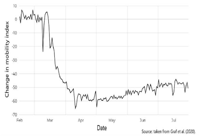
Although quantifying the causal link between mitigation policies and actual social distance is out of the reach of this paper, there is some evidence that mitigation measures have been effective. Figure 1 reproduces a mobility index constructed by researchers from the National Council for Science and Technology (Consejo Nacional de Ciencia y Tecnología, CONACYT, in Spanish) using data from social media (^{Graff et al., 2020}). According to this evidence, mobility declined more than 60% in April, compared to the pre-epidemic period. And, even after the end of Stage 3 and the gradual reopening of the economy starting in June, the most recent data shows still a reduced mobility of about 50%.

Figure 1 Mobility index 

In the following sections I provide estimates of the benefits of mitigation policies in terms of averted deaths and compare these benefits to the costs of the control in terms of aggregate output.

3. Projecting the size of the epidemic in Mexico

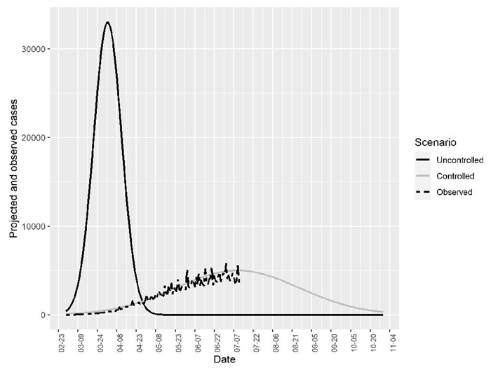
Predicting the final size of the epidemic is a difficult task, mainly because of the limited amount and characteristics of available data when the epidemic is still active. Also, all forecasts depend on the assumptions made on the population’s behavior and on the set of policies in effect. In this paper I do not attempt to make a projection of the size of the epidemic. Rather, I rely on two projections from the Health Secretary and CONACYT. According to a projection, if no actions were taken and the epidemic had occurred without control, the epidemic would have peaked around the first week of April, reaching a maximum of 33,000 new daily cases. On the other hand, another projection made by researchers at CONACYT (^{Quiroga et al., 2020}) implies that under the current scenario with mitigation measures the peak of the epidemic happened during the first week of July, with over 5,000 new daily cases.

I take the peak dates and the maximum number of daily cases at the peak as given and recover the full distribution of cases under the two scenarios.² I assume the uncontrolled and controlled peak dates are April 1 and July 10, respectively, and that peak heights are 33,000 and 5,000 cases, respectively, based on CONACYT’s projections (^{Quiroga et al., 2020})

I follow ^{Greenstone and Nigam (2020)} in assuming a normal distribution for the daily counts of cases (and deaths). For the uncontrolled scenario, I thus know x and φ(x) at two points, the peak and the first case date. Then, I solve for the value of the standard deviation σu that satisfies φ (Apr 21)=33,000 and φ (Feb 29)= cases0 . The implied standard deviation turns out to be σu =10.76. A similar procedure using the controlled scenario peak and date yields σc =47.55. In figure 2, I show the computed distributions of cases under the uncontrolled and controlled scenarios, together with the observed number of cases from the Health Secretary. The projected number of cases with mitigation closely follows the trajectory of the actual data.

Figure 2 Fitted cases distribution 

^{Greenstone and Nigam (2020)} follow a similar approach to approximate the U.S. deaths curves in ^{Ferguson et al. (2020)}. Ferguson and colleagues use primary data from China and other countries with early COVID-19 outbreaks, together with the distribution of cases across ages to estimate the expected number of cases and deaths in the U.S.and the U.K. Ferguson and coauthors estimated that 2.2 million people would have died in the U.S. without social distance measures, while 1.1 million deaths can be expected under the controlled scenario. Although ^{Greenstone and Nigam (2020)} did not have access to Ferguson’s data, they estimated almost the same number of deaths using normal approximations. Using a standard epidemiological SIR model, ^{Thunström et al. (2020)} obtain a similar estimate of 0.94 million deaths in the U.S. under the scenario with mitigation measures.

My estimates imply a total number of COVID-19 cases in Mexico of 889,468 in 2020 (assuming a single wave of contagion) under the uncontrolled scenario and of 594,372 under the controlled scenario of social distance and other mitigation measures. That is, mitigation measures reduce in 33% the total number of cases. I summarize these findings in table 1.

4. Estimating hospital and ICU demand

^{Ferguson et al. (2020)} estimate that about two thirds of COVID-19 cases are not severe and do not require hospitalization. This figure is close to the fraction of hospitalized patients in the data from the Mexican Health Secretary. Thus, to estimate the demand for a hospital bed in Mexico, I use Ferguson’s proportion (0.33) for both the uncontrolled and controlled scenario.

Similarly, according to ^{Wu and McGoogan (2020)}, up to 5% of COVID-19 cases require ICU, which might include a ventilator. With these two proportions, an estimate of daily and accumulated demands for hospital beds and ICUs can be computed. Table 2 shows the results of these calculations. I estimate that 293,524 patients would need a hospital bed and over 44,473 would require an ICU under no mitigation measures. These figures decrease to 196,143 and 29,719 with mitigation policies. Thus, mitigation measures reduced total healthcare demand by 33% and demand at the most critical date by 85%.

These calculations are crucial for estimating the daily fatality rates since the survival probability depends in part on whether the indicated healthcare is received or not. In the following section, I calculate the availability of healthcare resources to project the expected daily supply of beds and ICUs.

5. Healthcare supply

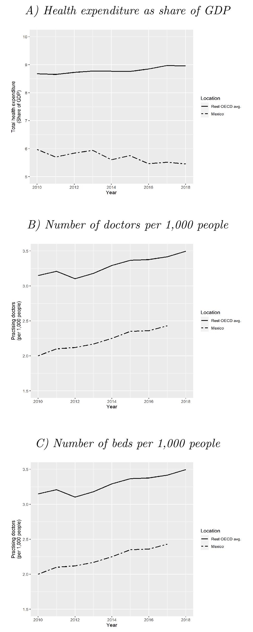
The COVID-19 epidemic highlighted the structural deficiencies of the Mexican healthcare system. Over the last 10 years, the total expenditure on health in the economy has remained about constant and represents only 60% of the average expenditure in the OECD countries. During the same period, the stock of resources in per capita terms has also remained almost unchanged. Figure 3 presents three indicators that contextualize the difference in the amount of healthcare resources that can be made available in Mexico during the epidemic.

Source: World Bank (2020).

Figure 3 Comparison of three health indicators for Mexico and the rest of OECD countries 

In order to respond to the COVID-19 epidemic, the public and the private sectors have redirected an enormous amount of resources. The availability of resources is extremely important since the survival probability of COVID-19 patients depends mainly on demographic factors, the presence of comorbidities, and, critically, on the provision of adequate specialized care when indicated.

I rely on several sources of data to approximate the total stock of hospital beds and ICU facilities that would be available for COVID-19 patients during the epidemic. According to ^{OECD (2019)} figures, there are 1.4 beds per 1,000 inhabitants in México, the lowest for any OECD member country. Nevertheless, not all these beds are properly hospitalization beds. Using official data from ^{Secretaría de Salud (Health Secretary) (2020a)} Catalog of Health Establishments (CLUES), I calculate a stock of 123,214 hospitalization beds (including both, private and public sectors) or about 0.96 beds per 1,000 inhabitants, 31% less than OECD figures.

For the stock of ICUs, I rely on ^{Secretaría de Salud’s (2020b)} Health Resources open data. According to this source, there are 3,800 ICU beds in Mexico. Furthermore, over the course of the epidemic, the private sector announced it would put at government’s disposal more than 3,000 hospital beds and 500 ICUs. This increases notably the capacity of the health sector for handling the epidemic. ³

To convert the stocks of beds and ICUs to daily availability, one must consider that most of the healthcare resources are always in high demand. Governments have tried to get around this allocation problem by postponing elective treatments to free physical and human resources. ^{Greenstone and Nigam (2020)} estimate that up 37% of ICU beds in the U.S. can be made available for treating COVID-19 patients. ^{Moghadas et al. (2020)} use a 65% availability to project COVID-19-induced demand for hospitalization beds in the U.S. Nevertheless, the health system in Mexico is likely to be under higher demand. According to ^{OECD (2019)}, the bed occupancy rate in Mexico is 74%. In this paper, I will assume a 25% availability rate for both hospital beds and ICUs.

Daily bed availability depends also on the number of days each resource is used. ^{Ferguson et al. (2020)} and ^{Greenstone and Nigam (2020)} assume every ICU patient uses a bed for 12 days, somehow lower than the reported hospitalization duration of 15 days in Hong Kong, Japan, Singapore, and South Korea (^{Gaythorpe, 2020}). ^{Guan et al. (2020)} estimate that the average hospital stay is 12 days long. In this paper I assume an average length of use of 12 days.

A final piece of information needed to project the daily supply of hospital beds is that the estimated stock (123,214) is dispersed around all of types of medical specialties, so not every bed can be considered as appropriate for treating COVID-19 patients. Using the Secretaría de Salud’s (2020) Health Resources open data (with data only available for public health units), I present in table 3 the share of beds in each medical specialty. I assume that 50% of the available stock of beds can be used or modified to receive COVID-19 patients, mainly considering that even if the physical capacity could be easily converted, it is difficult to think that the highly specialized medical personnel necessary for treating COVID-19 patients can be properly trained quickly enough.

With the estimated stock of beds and ICUs and the estimated unoccupied shares, the amount of resources made available by the private sector, and the average number of hospitalization/ICU days, I can calculate the daily availability of hospital beds and ICUs for treating COVID-19 patients. Table 4 summarizes this information. The daily supply of hospital beds and ICUs defines a threshold (surge capacity) above which hospitals cannot meet demand and the system becomes overcrowded.

6. Projecting excess of demand

Using my estimates on the daily supply of hospital beds and ICUs, together with the projected demand for hospitalization and critical care, I estimate the excess demand that would have occurred in the uncontrolled scenario and the date of this happening. Figure 4 represents this allocation problem. The dashed lines show the amount of resources available at every moment, while the solid curves are the estimated demand derived in section 4. At the beginning of the epidemic, the system can provide care according to the total hospital bed and ICU availability (18,402 and 1,450 units, respectively). As the infection progresses, demand grows fast exhausting medical resources as they reach the surge capacity. As is evident from figure 4, the number of patients requiring a hospital bed or an ICU would have exceeded the supply as early as by the second week of March. By the time of the projected peak date (April 1st), the system would have required almost 11,000 hospital beds and 1,600 ICUs every day.

Figure 4 Projected supply and excess of demand, uncontrolled scenario 

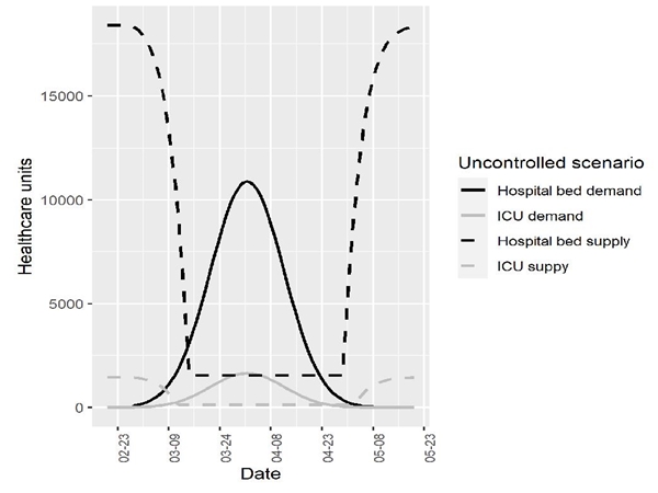
The area between the supply curve and the projected demand represents the unmet demand and thus, the number of patients that face a challenge to their survival probability.

On the other hand, under the controlled scenario of mitigation measures, figure 5 depicts a much different situation. One of the main objectives of these paper is to quantify the benefits of social distance and other mitigation policies by reducing the pressure on the healthcare system. Under this situation, the demand for hospital beds would have exceeded the supply starting June 22, while the demand for ICUs would exceed the supply more than a month earlier, by May 16. The differences in areas between the supply and demand curves across scenarios provides a measure of one of the most important benefits of flattening the curve.

Figure 5 Projected supply and excess of demand, controlled scenario 

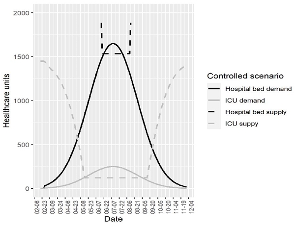
I estimate that the social distance measures reduced hospital bed excess of demand by over 200,000 cases and ICU excess of demand by over 28,000 cases. Still, even under the controlled scenario, more than 2,800 patients that are indicated hospitalization are denied it, and about 9,000 patients in urgent need for ICU do not receive the appropriate care (table 5). It is important also to note that under the controlled scenario, the number of days the demand for hospital beds is above the supply is practically the same as under no control measures (37 and 39, respectively). On the other hand, the period of overcrowded ICUs is almost three times larger. This means that flattening the curve can also translate into some resources being used for longer. Thus, the number of days in which demand exceeds capacity is not in all cases the best indicator for mitigation success.

7. Estimation of daily deaths flow

One of the most important consequence of an overwhelmed system is that fatalities increase when appropriate care is not provided. Daily demand for hospitalization beds can be met until hospital bed supply reaches its surge capacity of 1,533 units. ICUs daily supply at surge capacity is 121 new daily cases. I use the projected demand and supply, and the number of cases denied appropriate treatment to project the daily flow of fatalities.

If ICU is indicated and the system is below surge capacity, the survival probability is 50% (^{Wu and McGoogan, 2020}; ^{Greenstone and Nigam, 2020}). On the other hand, with the system above surge capacity, patients that require an ICU and do not get appropriate treatment have a 10% survival probability (^{Ferguson et al., 2020}; ^{Greenstone and Nigam, 2020}).

Patients that are indicated hospitalization but not ICU have better prospects, also depending on the received healthcare. According to the observed data from Mexico 34% of hospitalized patients have died. Thus, I use 66% as an estimate of the survival probability when the system is below surge capacity. For an overwhelmed system, I assume the fatality probability doubles for patients who are denied care.⁴

Finally, I assume a 99% chance of surviving for COVID-19 ambulatory cases (the observed survival rate in the data is 98.28% of ambulatory cases). In table 6, I summarize the parameters used to calculate the daily flow of deaths.

Figure 6 presents the results of my estimates of daily deaths flows, together with the observed number of deaths for 2020. Under the uncontrolled scenario, the accumulated number of deaths would have exceeded 214,000. On the other hand, under social distance and mitigation measures, the number of deaths is expected to be reduced to about 90,000. Under the uncontrolled scenario, a maximum of 8,525 daily deaths would have been expected versus a maximum of 808 daily deaths under the current controlled scenario.

Figure 6 Projected and observed deaths 

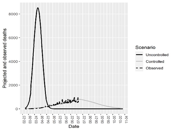
I summarize these findings in table 7. Flattening the curve lowers the death toll by 58%, not only because less cases occur, but because the disease spreads over a longer period, reducing daily pressure on the healthcare system and making it less likely that patients are denied the indicated healthcare, avoiding a considerable drop in the survival probability.

Put another way, 237,397 more patients face a hike in their probability of dying in the uncontrolled scenario. The benefit of social distance measures is 167,629 patients who would have otherwise died due to overwhelmed hospitals.

8. Monetizing the benefits of mitigation measures

Public policies aimed at reducing fatalities or damaged health include in their cost-benefit analysis an estimate of the willingness to pay for a reduction of the risk of death. A standard measure of the value of this reduction is the value of a statistical life (VSL), which represents an individual’s willingness to pay in dollars for a marginal change in her own risk of dying (typically a 5 in 10,000 change) in a year (^{Robinson et al., 2019a}). The VSL concept is sometimes wrongly understood as the value that oneself, the analyst or a government assigns to a human life. Rather, the concept must be interpreted as the rate at which an average person considers a dollar available for spending equivalent to a reduction in her mortality risk (^{Robinson et al., 2019b}). A typical VSL value for evaluating mortality risk reductions in the U.S. is 10 million USD.⁵

Direct estimates of the VSL from a population are usually obtained by linking occupational risks and wages or by extracting values from stated valuations surveys. In the absence of recent estimates for Mexico, I rely on an alternative strategy of benefits transfer. The benefits transfer methodology takes a base estimate of the VSL from a country with reliable data (A) to extrapolate the VSL to country B, adjusting by the differences in income between the two countries, according to the following expression:

where δ is the income elasticity. To obtain an estimate of the VSL for Mexico, I use a VSL estimate for OECD countries of 3.83 million USD in 2011 (^{OECD, 2012}). I use the per capita GDP (PPP) from the IMF’s World Economic Outlook to calculate an income ratio of 0.44 and assume an elasticity of 1.1.⁶ Following this procedure I estimate a VSL for Mexico of 1.8 million USD.

Table 8 summarizes the second set of main findings of this paper. The reduction of deaths due to the mitigation policies represents a benefit of 224,500 million USD. In line with ^{Greenstone and Nigam (2020)}, I label this figure as the direct benefit. Additionally, social distance and mitigation measures have an indirect effect in reducing hospitals and ICUs overcrowding, generating an additional benefit of 301,732 million USD. The total benefit of mitigation measures amounts to 536,232 million USD.

9. Mitigation costs and net benefits

The total economic effect of the COVID-19 epidemic in Mexico is as difficult to forecast as the duration of the pandemic itself. New waves of contagion or a too-early lift of restrictions could lead to a new set of mitigation measures that make the cost higher. Moreover, together with the direct effects of the epidemic, the Mexican economy faces an adverse future scenario in which important sources of revenues, such as tourism, remittances, and the oil industry, are expected to perform badly. These factors will influence the depth of the downturn and the speed of recovery.

How large are the benefits from mitigation measures estimated in earlier sections? From an ethical point of view it could be argued that any dollar spent to avoid deaths is worth it. But since mitigation policies involve a high economic cost, we can approximate the implicit value that the society or a government puts on saving lives by performing a cost-benefit analysis.

To estimate the magnitude of mitigation costs I rely on potential recovery scenarios estimates constructed by the Bank of Mexico (^{Banco de México, 2020}). Figure 7 depicts the shapes of the different trajectories. In my cost-benefit calculations the cost is defined as the accumulated output gap from the first quarter of 2020 (when output starts declining) up to the date when the output catches up the business-as-usual trajectory. The business-as-usual trajectory is constructed by assuming a constant 2% annual growth and represents the expected trajectory that output would have followed in the absence of health and economic shocks. The Bank of Mexico projects trajectories until the end of 2021. I complete the trajectories making some plausible assumptions summarized in table 9. The uncontrolled scenario is constructed by assuming that output falls only two thirds of what it would fall under the V-shape recovery scenario.

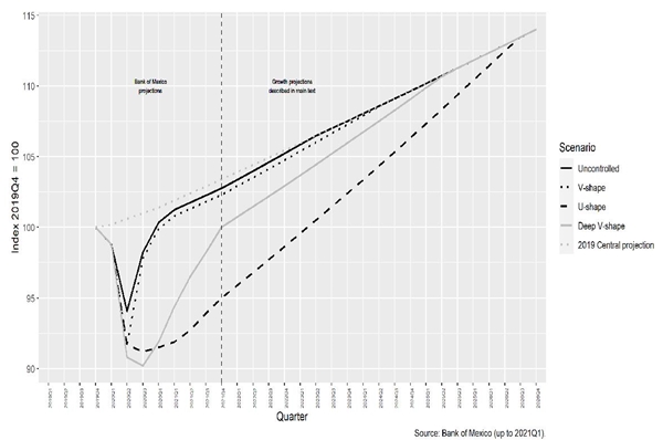
Figure 7 Projected output gap under the uncontrolled scenario and under different recovery scenarios 

For each recovery trajectory, I calculate the present value of the stream of quarterly gaps with respect to the business-as-usual trajectory. To discount future flows, I use a discount rate of 5%. The difference between the uncontrolled recovery trajectory and each of the controlled trajectories is the measure of the cost of mitigation policies. Table 10 presents the third set of key results of this paper.

Under the scenario with no mitigation policies, the output gap accumulated from 2020-Q1 to 2023-Q2 equals 401 billion USD (15% of Mexican GDP in 2019). I compare this estimate to the gap under each of three alternative controlled recovery scenarios. A fast recovery, represented by the V-shape recovery scenario, implies that an uncontrolled pandemic scenario would cost 208 billion USD. On the other hand, the U-shape recovery scenario, caused by mitigation efforts, costs 2,992 billion USD. The deep V-shape scenario, consistent with the IMF’s projected GDP fall in 2020, represents a cost of control of 1,444 billion USD.

The net benefit of mitigation measures is the difference between the monetized benefits of averted deaths and the cost of control. Only the V-shape fast recovery scenario yields a positive net benefit (12% of GDP). For the U-shape scenario, the (negative) net benefit of mitigation measures is 2,466 billion USD (95% of GDP), while under the deep V-shape scenario, the (negative) net benefit would be 918 billion USD (35% of GDP).

The negative net benefit does not necessarily mean it would be rational to opt for the uncontrolled scenario. Instead, my interpretation is that this partially reveals the implicit benefit that the society and the government assign to avoiding the consequences of the uncontrolled scenario (loss of reputation, political instability, and social chaos, among others). Another alternative explanation is that the society reveals with its mitigation actions that it values the probability risk reduction of a given individual more than the individual’s own valuation (a typical externality problem).

Following this reasoning, I calculate two additional indicators. First, I compute the break-even number of total averted deaths, which represents the sum of direct and overflow deaths that would compensate the cost of control. That is, if the society or the government only valued the lives saved according to the VSL, this figure gives the number of averted deaths that equalize the cost of control. Under the slow recovery U-shape scenario, more than 1.6 million deaths would need to be averted to compensate the cost.

Second, I compute the break-even VSL, interpreted as the VSL that compensates the accumulated output gap over the recovery period given the 292,351 averted deaths under the controlled scenario estimated in section 8. A fast recovery (V-shape) would require a VSL of only 0.71 million USD. On the other hand, with a U-shape recovery, the VSL should be 10.21 million USD, a figure similar to the one used in the evaluation of distinct policies in the U.S.

A last observation on the different recovery trajectories deserves to be discussed. The V-shape results in this paper can also be interpreted as what could be achieved if fiscal and monetary policies were used to put the economy on a much faster recovery trajectory. Governments around the globe have implemented measures to guarantee workers income and to compensate firms for their revenue losses. The economic policies implemented by the Mexican government have been rather moderate, relying on the set of already existing programs. However, most of these programs are likely to exclude urban and informal workers and enterprises. Furthermore, the federal government has cut its own materials and operation costs budget for the reminder of the year, while federal employees remain working remotely.

There is no clear relationship between the size of the fiscal efforts and the expected fall in GDP, at least for Latin American countries (^{Esquivel, 2020}). This fact can be explained by the nature of the economic downturn, characterized by negative shocks on both demand and supply (^{Guerrieri el al., 2020}). Therefore, expansionary fiscal policies are likely to be ineffective during the epidemic even if households are willing to spend and even if governments stimulate aggregate demand. Nevertheless, a lack of policies that guarantee the survival of small and medium businesses and that prevents workers from falling into poverty compromises the prospects of a recovery once restrictions to mobility and economic activity are lifted.

10. Sensitivity analysis

One disadvantage of the previous analysis is that it is mostly deterministic. I borrow most key parameters from an emerging literature and complement some of the missing information with the early data from Mexico to project the trajectories of cases, resource utilization and deaths. Also, my analysis does not allow for uncertainty in the recovery trajectories once one of them is chosen for comparison to the uncontrolled scenario. Thus, to analyze the sensitivity of my results and to emphasize the channels through which key parameters operate, I performed the same analysis described in this paper, changing one of the key parameters one at a time.

Thus, I present in table 11 a summary of the consequences of deviating from the parameters assumed in the earlier sections of this paper for the controlled scenario (the uncontrolled scenario remains the same) in terms of cases, deaths, days of overflown healthcare system, and monetized control benefit. I also present the net benefit, the break-even VSL, and the break-even death toll for each of the recovery trajectories. For each alternative parameter specification, I compare what the controlled scenario achieves with respect to the uncontrolled one. The first line of this table summarizes the findings described earlier in this paper. The mitigation strategies reduce the number of cases by 33% and the number of deaths by 58%. There are 5% less days of overcrowded hospitals and 146% more days of overcrowded ICUs. The mitigation policies reduced overflow deaths in 94%. The benefits of flattening the curve are monetized as 526 billion USD.

If we assume a better control strategy in which the peak of the controlled curve is of only 2,500 cases, the number of total cases would be much smaller (63% reduction, compared to the uncontrolled scenario). Under this alternative assumption, the healthcare system would be under considerably less pressure: there would never be overcrowded hospitals and the number of days with overcrowded ICUs would be reduced by 41%, compared to the uncontrolled scenario. A fast V-shape recovery would yield a positive net benefit of 414 billion USD. Nevertheless, the other two slower recovery trajectories imply net costs not very different to the net costs in the main results of the paper.

The assumption on the percentage of total beds that can be converted for treating COVID-19 patients is an important one and the consequences of different probabilities deserve to be discussed. A larger probability of conversion can also represent a scenario where the initial bed and ICU availability was higher at the beginning of the epidemic. As I report in section 5, the overall expenditure in the health sector and the amount of healthcare resources in Mexico have remained considerably below than the average OECD country. Thus, an increase in the probability of conversion to 75% also represents a situation in which the initial available stock of hospital beds for providing adequate care to COVID-19 patients is 26,103 rather than 18,402. Also, the surge capacity would be increased to 2,175 beds under this alternative assumption.

The results from this experiment show the following: since more beds are available at the beginning of the epidemic, it is more likely that even under the uncontrolled scenario more people receive appropriate healthcare. Under the new controlled scenario, with more beds available, there are no days in which the hospital beds’ demand exceeds the supply. Nevertheless, the monetized benefit of the control is only 483 billion USD (compared to the 526 billion USD in the main results of the paper). Thus, the net benefit of a fast V-shape recovery is lower and the negative net benefits under the U-shape and deep V-shape recoveries are greater. Put in other words, had the initial resources been sufficient for better handling the epidemic, a controlled scenario as costly as those represented by the U-shape or the deep V-shape trajectories could have been avoided.

If we now assume a larger fraction of cases were severe enough to need an ICU (10%, twice as large than most estimates in the literature), the number of days the ICU capacity is overcrowded increases 204%. In such a case, the benefits of control are more evident and the net benefit of control under a fast V-shape recovery increases to 374 billion USD. Similarly, the negative net benefit in the two slowrecovery scenarios is lower than in the main results of the paper. If we assume a bed is used for 18 days, the control is less effective in terms of lives saved, while the healthcare system would be overcrowded for many more days, reducing the net benefits of control.

Finally, assuming a higher interest rate in the valuation of the future output gap in section 9 does not alter the epidemic outcomes but increases the net benefits of control as future streams of output are discounted at a higher rate.

11. Conclusion and agenda

The main objective of this paper has been to organize the discussion on some of the factors that affect the effectiveness of mitigation interventions and to provide a quantitative assessment of some of the economic benefits of flattening the epidemic curve. In this paper I estimate the daily flows of cases under the scenario of social distance and restricted economic activity implemented during the first months after the beginning of the epidemic, and under a counterfactual uncontrolled scenario with no mitigation measures. I quantify the supply of hospital beds and ICUs and project the number of deaths under both scenarios. I estimate that social distancing measures reduced the number of COVID-19 cases by 33%. The benefits of mitigation measures amount to a direct reduction of 124,722 direct fatalities and of 167,629 deaths avoided by reducing the exerted pressure on the healthcare system. The benefits of these measures are monetized as 526 billion USD.

In the absence of treatments and vaccines, mitigation measures to control the COVID-19 pandemic are likely to produce vast economic impacts. I calculate the costs of control measures as the output gap from the first quarter of 2020 until the date when the recovery trajectory reaches the output expected before the epidemic, in the absence of health and economic shocks. Under a plausible recovery scenario, mitigation measures will have net costs of 35% of the Mexican GDP in 2019. On the other hand, under a less likely fast V-shape recovery, the net benefits from mitigation measures in Mexico would represent up to 15% of 2019 Mexico’s GDP. The costs of control can be reduced if the mitigation measures reduce the number of cases by more than what is projected or if more resources become available to avoid the overcrowding of the healthcare system. Also, a lower cost can be attained if a faster recovery occurs or if the government stimulates the economy enough to reduce the output gap.

The V-shape results in this paper can also be interpreted as what could be achieved if fiscal and monetary policies were used to put the economy on a much faster recovery trajectory. The economic response by the Mexican government has relied on the set of already existing programs, which are likely to exclude support for urban and informal workers and enterprises. A lack of policies that guarantee the survival of small and medium businesses and that prevents workers from falling into poverty compromises the prospects of a recovery once restrictions to mobility and economic activity are lifted.

Some limitations of my analysis deserve to be discussed for future research. In this paper, I assume that the differences in fatality rates for patients that receive appropriate healthcare versus those who are denied it are independent of the age profile. ^{Verity et al. (2020)} have shown that fatality rates differ across age groups. A recent debate on the ethical dimension of assigning medical resources questions whether younger patients should be allocated for treatment first. In my calculations I have implicitly assumed random assignment of patients to healthcare in case of overflow. If one assumes some form of sorting in the assignment, the net cost of the control is likely change. Studying the implications of different rules for assigning patients is part of an open agenda.

In this paper, as in other analyses at an aggregate level of healthcare resources, an implicit assumption is that patients from all over the country can be allocated to a hospital bed or ICUs if required, if an ICU bed is available anywhere in the country. A more detailed analysis would utilize state or city specific projections of the epidemic and regional supply of resources, together with transaction costs. Unfortunately, the necessary data to make reliable local predictions on the epidemic progression and the local availability of health resources is not currently available.

Finally, my calculations imply that under plausible recovery scenarios, the net benefits of control are negative. If this is the case, we need to understand the factors that make societies and government willing to incur the cost of control. For example, societies may be willing to pay more than an individual is to reduce mortality risks if everyone generates positive externalities. Alternatively, a government is likely to assign a very large cost to the political consequences of an uncontrolled epidemic.