SciELO - Scientific Electronic Library Online

 
vol.67 número4Brownian motion and polarized three-dimensional quantum vacuumPrediction of electronic and optical properties for Zn1−x Cdx Sey Te1−y quaternary alloys: First-principles study índice de autoresíndice de assuntospesquisa de artigos
Home Pagelista alfabética de periódicos  

Serviços Personalizados

Journal

Artigo

Indicadores

Links relacionados

  • Não possue artigos similaresSimilares em SciELO

Compartilhar


Revista mexicana de física

versão impressa ISSN 0035-001X

Rev. mex. fis. vol.67 no.4 México Jul./Ago. 2021  Epub 14-Mar-2022

https://doi.org/10.31349/revmexfis.67.040801 

Research

High Energy Physics

Lepton flavor violating hτµ decay induced by leptoquarks

M. A. Arroyo-Ureñaa 

R. Gaitána 

J.H. Montes de Ocaa 

R. Sánchez-Vélezb 

aDepartamento de Física, FES-Cuautitlan, Universidad Nacional Autónoma de México, 54770, Estado de México, México.

bFacultad de Ciencias Físico-Matemáticas, Benemérita Universidad Autónoma de Puebla, 72570, Puebla, Pue., México.


Abstract

The flavor, changing neutral current decay hτµ is studied in a renormalizable scalar leptoquark model with no proton decay. Analytical expressions for the one-loop level contributions of a scalar leptoquark to the decay width of the process hτµ are presented. We find a viable model parameter space via the current constraints on the muon (g − 2), the decays τµγ, µ, the LHC Higgs boson data and the direct leptoquark searches at the LHC. Then, we evaluate the branching ratio of the decay hτµ induced by leptoquarks, which is of order 10−9 −10−7. We find that with the branching ratio so suppressed, it will be difficult to observe the hτµ decay in current colliders, but potential evidence could be observed at the Future hadron-hadron Circular Collider.

Keywords: Rare Higgs decays; scalar leptoquarks; flavor violating processes

1. Introduction

Once the Higgs boson was discovered at LHC by ATLAS and CMS collaborations [1, 2], several phenomenological studies on Higgs physics were proposed, from high precision experiments to processes that would indicate physics beyond the Standard Model (SM). In this context, nonstandard Higgs couplings, including the Lepton Flavor Violating (LFV) ones, are predicted by many models of physics beyond SM [3-8]. In particular, neutrino oscillations are a consequence of their massive nature, which is not addressed by the SM. The experiments with atmospheric, solar, reactor and accelerator neutrinos have provided evidence of this phenomenon [9-16], which motivated the occurrence of LFV in nature. In the framework of the SM, LFV processes vanish at any order of perturbation theory, which encourages the study of SM extensions that predict sizable LFV effects that could be at the reach of detection. In addition to decays as liljγ and liljlk¯lk, particularly interesting is the decay hτµ, which was studied first in Refs. [17-19]. Subsequent studies on its detectability appeared soon after [20, 21], which motivated a plethora of analysis in the context of several SM extensions [22-28], where the authors of Ref. [22] gave the first correct prediction, including the GIM-like suppression of this observable in the presence of right-handed neutrinos.

Searches for the LFV decay hτµ carried out by CMS and ATLAS collaborations in the τµ and channels were presented. However, no significant excess over the SM expectation was observed [29, 30]. The upper limits, at 95% confidence level, are:

CMS:BR(hτμ)<0.25%,

ATLAS:BR(hτμ)<0.28%.

With these encouraging values, searches for the LFV decay hτµ look promising with luminosities and energies larger than the one searched at the Large Hadron Collider (LHC). This could be achieved at future super hadron colliders, namely, High Luminosity LHC (HL-LHC) [31], High Energy LHC (HE-LHC) [32], and at Future hadron-hadron Circular Collider (FCC-hh) [33], which will reach an integrated luminosity of up to 3 ab−1, 12 ab−1 and 30 ab−1 and center-of-mass energies of 14, 27 and 100 TeV, respectively.

In our research, we study the decay hτµ in the framework of a specific version of Leptoquark (LQ) models, as presented below. LQs can be scalar or vector particles that simultaneously carry lepton and baryon number and can appear naturally in grand unified theories based on SO(10) [34,35], SU(5) [36] and SU(6) [37], as well as in the context of a SU(4) R ×SU(4) L ×SU(40) theory, where the lepton number is considered as a fourth color [38, 39]. These particles also appear in other extensions of SM, such as Technicolor [40,41], supersymmetric models with R-parity violation [42], models with composite fermions [43-45], etc. The LQs may or may not have well-defined baryon (B) and lepton (L) number; however, those with violating interactions can mediate the proton decay unless an extra symmetry is invoked to forbid the diquark couplings, otherwise the leptoquark masses are expected to be at the Planck scale to ensure the stability of the proton [46]. The low-energy LQ phenomenology has received considerable attention, and possible LQ manifestation in various processes has been extensively investigated [47-49]. The LQs with left and righthanded couplings to fermions are interesting candidates to explain the discrepancy of the muon anomalous magnetic moment (µAMDM) since they induce an enhancement by a factor m t /m µ ∼ O(103) or m b /m µ ∼ O(10) compared to the SM. Furthermore, the non-chiral LQs interactions can enhance as well the rare LFV Higgs boson decay hτµ.

The spirit of our work was essentially studied also in the Refs. [48,50,51], whose branching ratios BR(hτμ) are of order O(1%) because an explanation for an apparent excess of the BR(hτμ) reported by the CMS [52] and ATLAS [53] collaborations was provided. However, the authors of the aforementioned works carry out fine-tuning in order to explain the supposed excess, although nowadays it is ruled out. In our work, we take into consideration updated data, including the electron (g −2), which can be accommodated simultaneously with the muon (g−2) and the decays τµγ, µ.

The organization of our work is as follows. In Sec. 2, we briefly discuss the generalities of the LQ model that we are interested in Sec. 3. There is devoted on the constraints on the relevant model parameter space whose values will be used in our analysis. Section 4 is focused on the calculation of the LFV decay hτµ amplitudes and decay width. In addition, we present the number of signal and background events produced at LHC, HL-LHC, HE-LHC, and FCC-hh. Finally, conclusions and outlook are presented in Sec. 5.

2. Theoretical framework

It is quite feasible to study the low-energy leptoquark phenomenology in a model-independent way via an effective Lagrangian, under the assumption of renormalizability and SM gauge invariance. Deeper analysis about the most general effective interactions of scalars and vector LQs can be found in [46,54]. We focus on a simple renormalizable LQ model, where a SU(2) doublet R 2 with quantum numbers (3,2,7/6) is added to the SM. With this unique representation, it is not necessary to implement additional symmetries that forbid the proton decay since R 2 does not couple to a pair of quarks. After the electroweak symmetry breaking, two LQs with fractional electric charges 2/3e and 5/3e appear, where the latter has non-chiral interactions to fermions; therefore, its contribution can improve the branching ratio of the LFV Higgs boson decay BR(hτμ) at the one-loop level. The phenomenology of this model has been studied in Refs. [47, 55] and more recently in Ref. [49] where constraints on the couplings to a lepton-quark pair were obtained through the analysis of the µAMDM and the LFV tau decay τµγ. We are interested in the contribution of the non-chiral leptoquark since it gives rise to a chirality-flipping term which is proportional to the internal quark mass that can enhance the Higgs boson decay hτµ. Although the complete expressions for the non-chiral LQ contribution to hτµ were obtained in [49], the aim of this work is the analysis of the signals events in the present and future colliders. For our calculations, we require the LQ couplings to fermions, the gauge bosons, and the Higgs boson, which can be obtained from the effective Lagrangians presented below.

The symmetries of SU(3) C ×SU(2) L ×U(1) Y allow the following zero-fermion-number interactions of the LQ doublet R 2 [54]

LF=0=h2LijR2Tu¯Riiτ2LLj+h2RijQ¯LieRjR2+H.c., (1)

where F = 3B+L is the fermion number, QLi and LLj denote SU(2) L quark and lepton left-handed doublets, respectively, whereas qRi and eRi are the corresponding singlet fields, with i and j the generation indices. h 2L,2R are, in general, the Yukawa couplings matrices.

After rotating to the LQ mass eigenstates Ω 2/3 and Ω 5/3 (where the indices refer to the electric charge of the two leptoquark states) via an unitary rotation, we obtain the leptoquark couplings to a quark-lepton pair

LF=0=e¯i(λLijPL+λRijPR)ujΩ5/3*+e¯iηRijPRdjΩ2/3*+H.c., (2)

where P L,R are the chiral projection operators. Since the flavor eigenstates were rotated to the mass eigenstates, the couplings λL,Rij and ηRij already encompass such information. In order to avoid the very stringent constraints on the LQ couplings to fermions of the two first families in our study, we consider that Ω 5/3 only couples to the second and thirdgeneration fermions. On the other hand, the scalar leptoquark Ω 2/3 couples to down quarks-lepton pair, inducing the decay b at one-loop level. However, we are interested in the effects of the non-chiral LQ Ω 5/3 on the FCNC decay of the Higgs boson.

The leptoquark coupling to the photon, which is necessary for the calculations of the µAMDM and the LFV decay τµγ, can be extracted from the leptoquark kinetic Lagrangian

LkinLQieQΩkΩkμΩk*Aμ+H.c., (3)

where QΩk stands for the leptoquark electric charge. Finally, the Higgs boson coupling to LQs can be obtained from the following renormalizable effective LQ interaction to the SM Higgs doublet Φ

L=(MR22+λR2ΦΦ)(R2R2), (4)

where MR2 is the LQ mass. Then, we derive the Higgs boson coupling to the LQ Ω k

LλΩvHΩk*Ωk. (5)

where we denote the dimensionless coupling associated with the Higgs-LQ interaction term as λ .

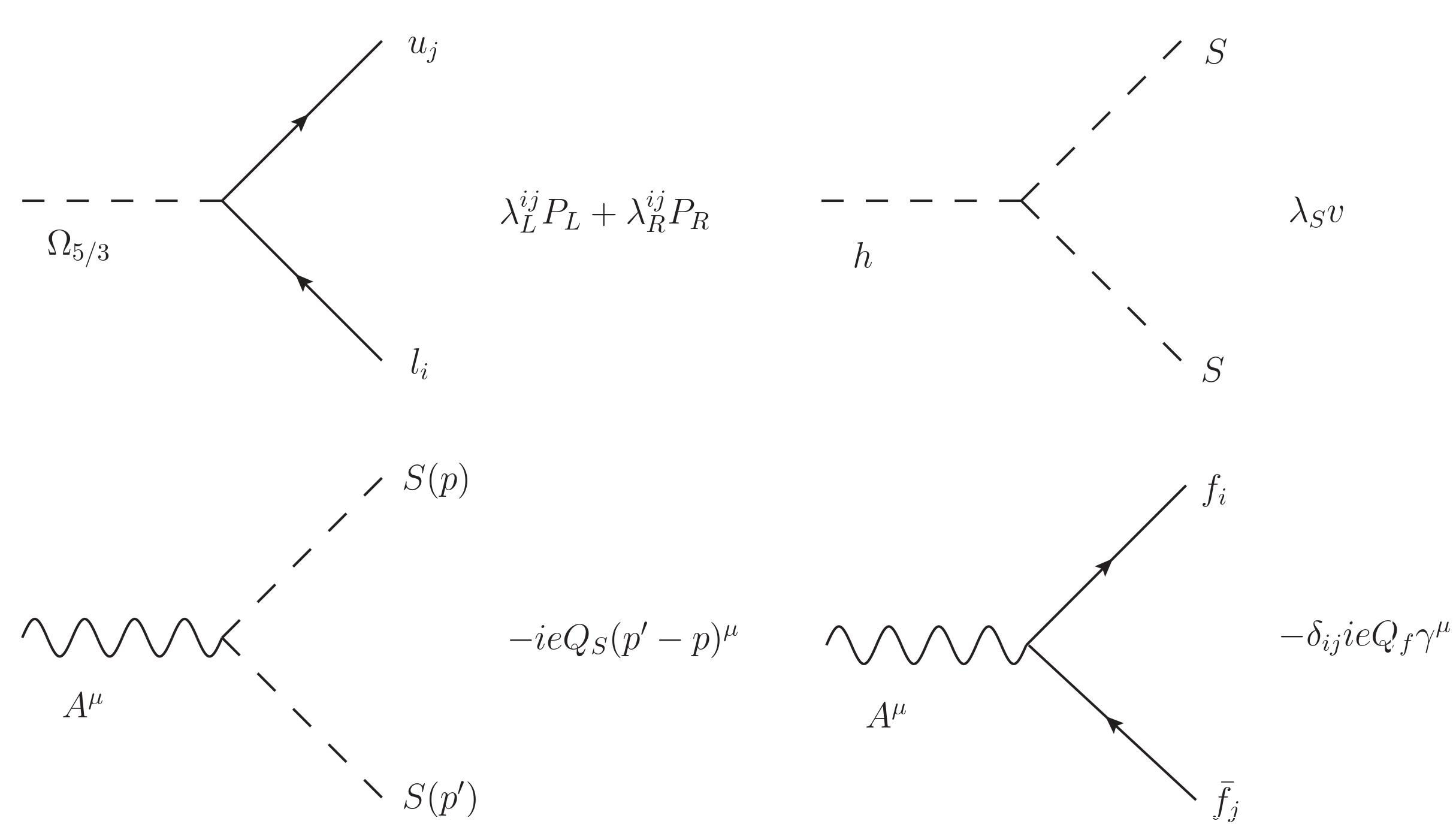
All the Feynman rules obtained from the previous Lagrangians are required for our calculations and can be consulted in Fig. 1.

FIGURE 1 Feynman rules for the couplings of the LQ to the pair lepton-quark, the Higgs boson, and the photon. For completeness, we also present the interaction of the photon with a fermionantifermion pair, where Qf stands for the fermion charge in units of the elemental charge. 

3. Constraints on the parameter space of the scalar LQ model

We now turn to the analysis of the parameter space for the LQ model previously introduced. We first start with a brief discussion about the constraints on the mass of the LQ and its coupling to the Higgs boson. Regarding the LQ coupling to fermions, we employ the µAMDM to constrain the LQ coupling to a µ-quark pair and the LFV decay τµγ to constrain the τ-quark ones. It turns out that low energy processes strongly constrain the couplings to the first-generation fermions while over the second and third-generations are less restricted.

Constraints on the mass for the LQs have been obtained by the ATLAS [56] and CMS [57] collaborations from the LHC data at s=13, where the most stringent value mΩ5/31 TeV, at 95% at confidence level (CL), was obtained assuming that the third-generation leptoquark Ω2 /3 mainly decays into a bottom quark and a τ lepton. Secondgeneration leptoquark pair production searches also give an upper limit, at 95% CL, of 1.5 TeV on the LQ mass [58]; however, we omitted that limit since Ω 2/3 couples to second and third-generation fermions. The leptoquark doublet R 2 can give large contributions to the oblique parameters unless the mass eigenstates Ω 5/3 and Ω 2/3 have a small mass splitting [59], then we will assume the bound m Ω5/3 ≥ 1 TeV in our analysis. On the other hand, the scalars LQs can considerably modify other loop-induced Higgs boson processes such as Hγγ and the production cross-section of the Higgs boson via the gluon fusion mechanism ggH. In particular, for the model, we are interested in the leptoquarks Ω 5/3 and Ω 2/3 that contribute to the loop functions and the corresponding LQ coupling to the Higgs boson λΩ=λΩ5/3=λΩ2/3 can be constrained by the so-called Higgs boson coupling modifiers. Such analysis was carried out in [49], where the coupling λ can take values in the interval (−5,5) for an LQ mass mΩ5/3=1 TeV. For larger values of the LQ mass, the allowed area slightly increases, being of order O(10); however, we will consider the conservative value: λ = 4, which agrees with the perturbative limit.

3.1. Constraints from the muon anomalous magnetic dipole moment and the LFV decay τµγ

The discrepancy between the theoretical and experimental values of the µAMDM has been a long-standing unsolved problem within the SM framework. On the theoretical side, the update SM theoretical prediction was reported in Ref. [60], whose value is aμSM=(116591810±43)×10-11. On the experimental side, the Brookhaven experiment E821 reports the value aμExp=(116592089±64±33)×10-11 [61]. These values yield to 3.7 σ level discrepancy

δaμ=aμExp-aμSM=(279±76)×10-11, (6)

that could be explained by the existence of new physics. In this work, we consider the leptoquark Ω 5/3 contribution as an explanation for the µAMDM. As pointed out before, the LQ mass must be rather heavy due to the LHC constraints; however, one can still get sizable effects in the µAMDM since the amplitude can be enhanced by the factor m t /m µ compared to the SM. As for the chiral leptoquark Ω 2/3 , its contribution to a µ is proportional to the muon mass and therefore subdominant. The scalar leptoquark Ω 5/3 induces the µAMDM at one-loop level via the Feynman diagrams of Fig. 2 for f i = f j = µ. Then, the contribution to a µ from LQ can be written as:

alLQ=-Ncml28π2q=t,c1mΩ5/32|λLlq|2+|λRlq|2I(xq)+mqmlReλLlqλRlq*J(xq), (7)

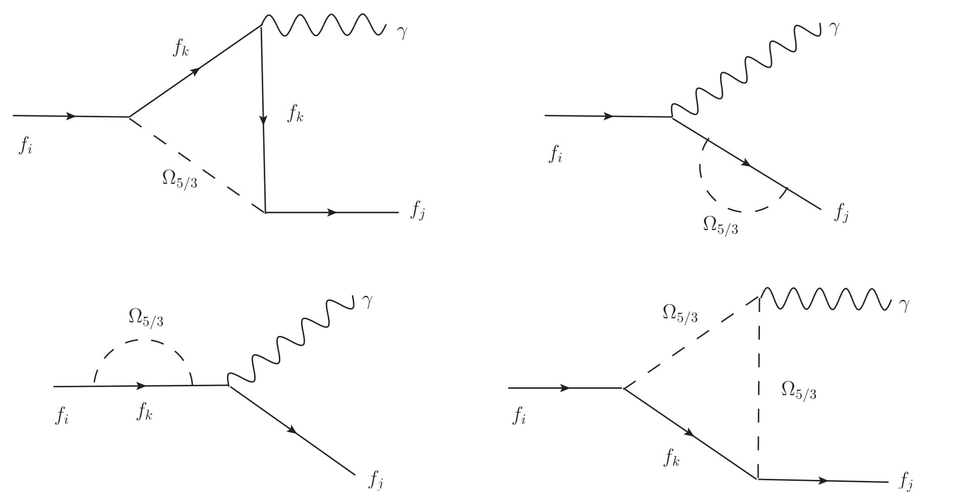
FIGURE 2 Feynman diagrams that contribute to the decay f i f j γ in the leptoquark model, where f i and f j can be leptons (quarks) if the internal fermion f k is a quark (lepton). The Ω 5/3 represents the leptoquark with electric charge 5/3 in units of the elemental charge e. Similar diagrams contribute to the µAMDM, only the replacement f i = f j = µ must be done. 

where N c is the color number of the internal fermion and l=e,μ,τ. The kinematic loop functions I(x q ) and J(x q ) depend on the variable xq=mq2/mΩ5/32, and they are given in Appendix A. It is interesting to note from Eq. (7) that the LQs having both left and right-handed couplings to charged leptons can generate much larger contributions due to the enhancement from the quark mass in the loop, mainly the top quark. If one assumes that the discrepancy δaμ is due entirely to the scalar leptoquark contribution aμLQ, we can obtain constraints on the leptoquark left and right coupling to the muon-quark pair λL/Rμq.

As for the constraints of the LFV processes, the experimental bound BR(τμγ)<4.4×10⁻⁸, obtained by the BaBar experiment, restricts the LQ couplings λL,Rτq and λL,Rμq. The Feynman diagrams for the LFV decay τµγ induced by the scalar LQ are shown in Fig. 2 for f i = τ and f j = µ. Just like the µAMDM, we only consider the leptoquark Ω 5/3 effects along with the top quark. We do not consider the charm quark since it gives a small contribution compared with the top quark.

The decay width for the process f i f j γ can be written as

Γ(fifjγ)=mi16π×(1-[mjmi]2)3(|L|2+|R|2), (8)

where form factors L and R are presented in Appendix B.

In order to explore the allowed values for the couplings λL/Rlt(l=μ,τ), we use the discrepancy of the µAMDM along with the experimental bound on the LFV tau decay. In Fig. 3, the allowed points in the plane λRtμλLtτ vs λLtμλRtτ are displayed for different values of the LQ mass. We observe that the leptoquark coupling products can be of the order of 10−3 for an LQ mass of mΩ5/3=2000 GeV; however, the allowed area slightly decreases when the LQ mass is mΩ5/3=1000 GeV. This behavior is understandable since the loop functions of the low energy processes are suppressed by the LQ mass and, therefore, larger areas for the LQ couplings are found when the LQ mass increases. Nevertheless, the Fermilab Muon (g−2) experiment [62], which will have four times the precision of the experiment conducted at Brookhaven National Laboratory, could confirm at a higher statistical significance the Brookhaven discrepancy with the SM. This would be a clear sign for physics BSM. Conversely, if the (g − 2) measurement confirms the agreement between measurement and SM theory, then this would place very strong limits on the existence of many BSM theories, such as the one considered in this paper. However, in our study, we are considering a scenario such that if the discrepancy disappears, our result would not be affected. On the contrary, we must wait for the update of the Fermilab Muon (g−2) collaboration and compare between the constraint imposed by the τµγ decay. This is because we find that this decay is more restrictive than δa µ .

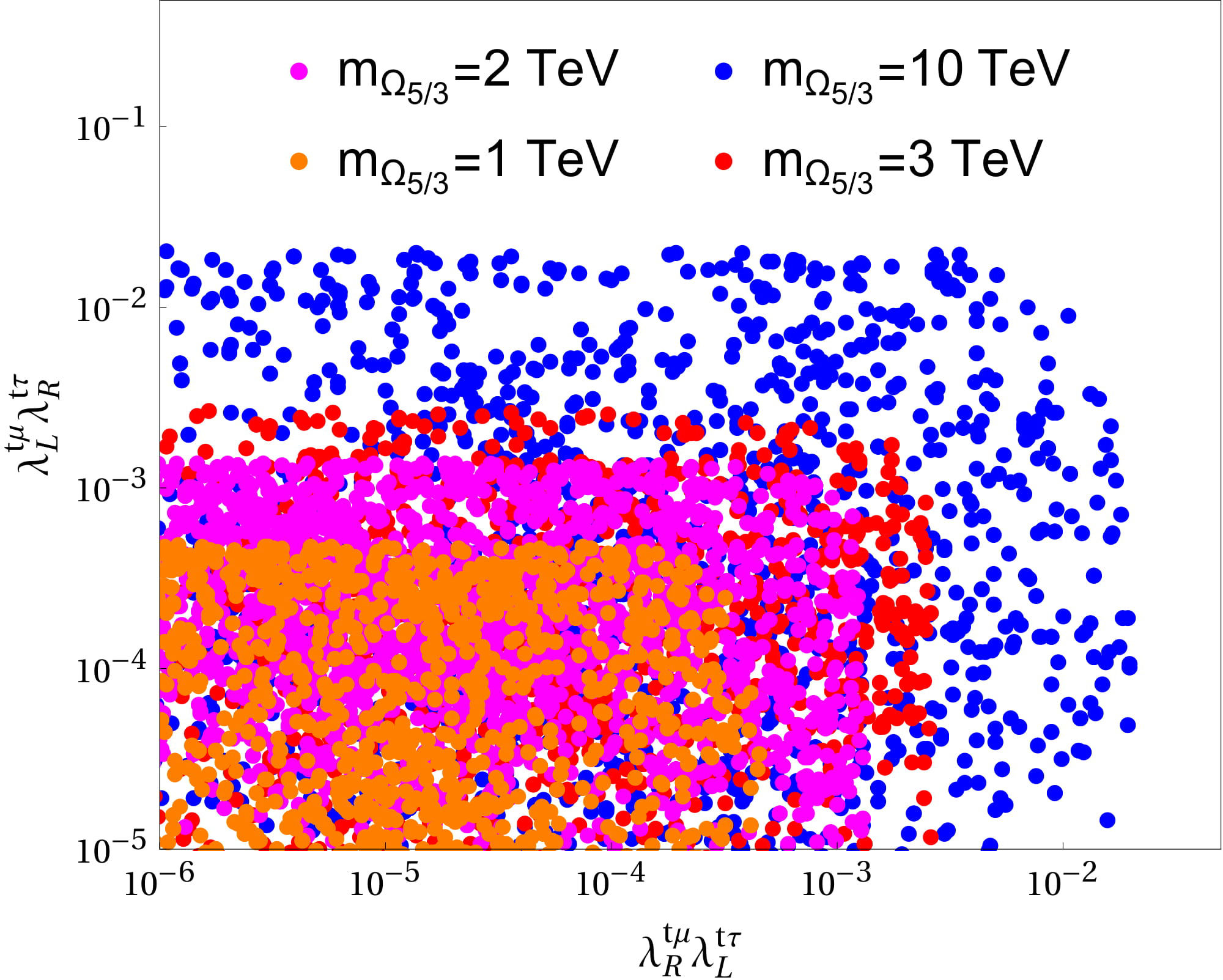
FIGURE 3 Allowed region in the λRtμλLtτ-λLtμλRtτ plane agree with the µAMDM and the experimental bound on the LFV tau decay τµγ for mΩ5/3=1 TeV (orange points online), mΩ5/3=2 TeV (magenta points online), mΩ5/3=3 TeV (red points online), mΩ5/3=10 TeV (blue points online). 

As far as the electron AMDM is concerned, the most current measurement of the fine structure constant α −1 = 137.035999206(11) [63] differs by 5.4 σ from cesium recoil measurement [64]. While the former is in agreement with the SM, the latter seems to point to a slight tension corresponding to a factor of 2.5. This controversy needs to be settled before concluding on the possible new physics BSM.

Given the above, it is worth mentioning that this model can simultaneously explain both the δa e (considering the result reported in Ref. [64]) and δα µ as well as the bounds on the BR of both µ and hµe. For illustration, we present in Fig. 4 the λLet-λLet plane, in which the blue points represent the ones that satisfy the upper limit on BR(μeγ) [65]; meanwhile, the red points represent the values for which δα e is corrected (in case of being preserved [64]). We do not include points for the decay hµe since it is easily explained in our theoretical framework.

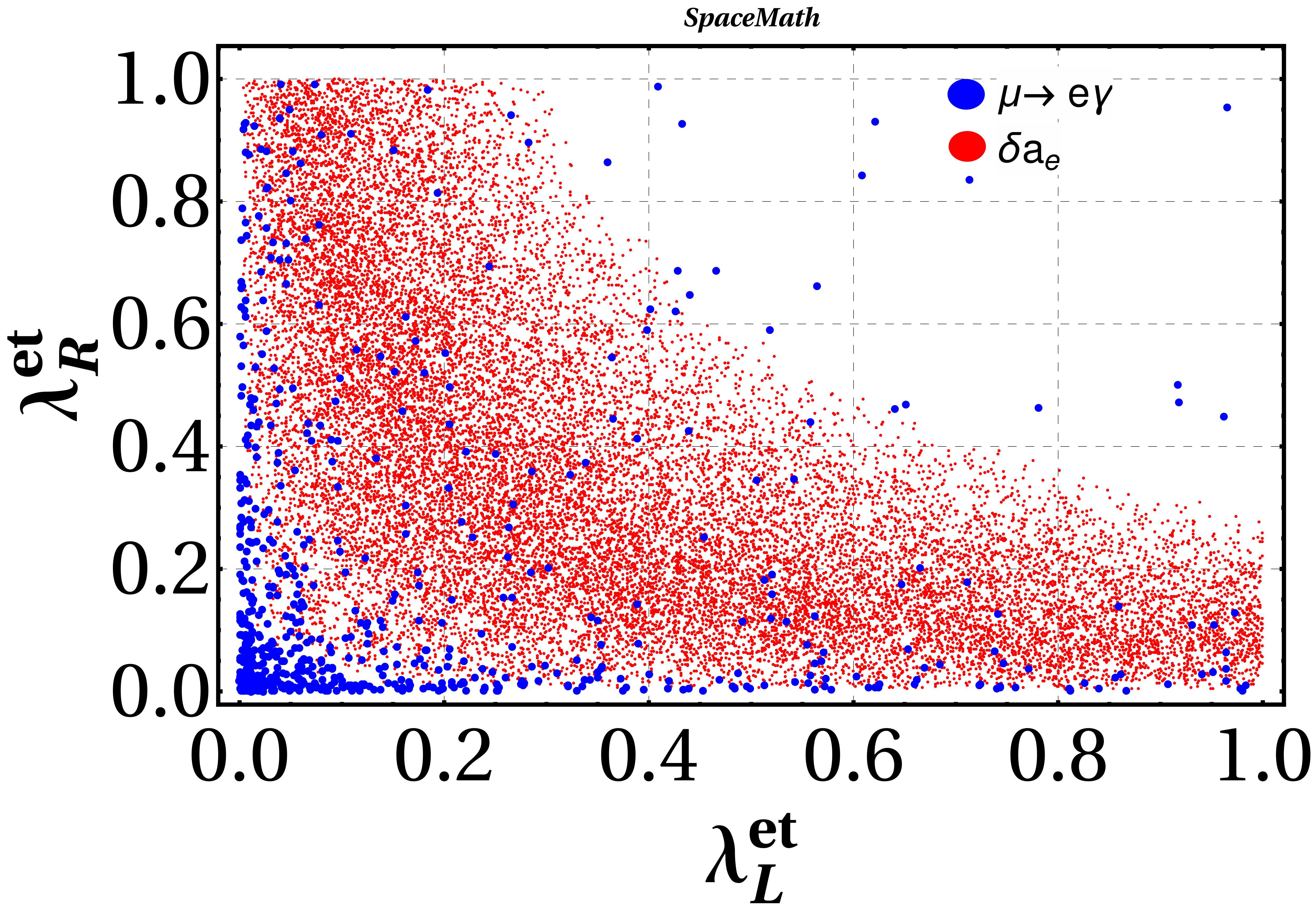
FIGURE 4 Allowed region by electron anomalous magnetic dipole moment δα e (red points) and the µ decay (blue points). 

The allowed region that satisfies both δα e and µ is the one in which the points overlap, and we observe that this allowed region is a combination of the values of λR,Let. For example, the values that accommodate δα e , setting λR,Let=10-6 (values that satisfy the upper bound on the decay µ), are in the interval (0.1-1). In an intermediate regime, we find values for λR,LetO(10-2) that explain both observables. The graph was generated by the SpaceMath package [66].

4. Decay hτµ induced via scalar leptoquarks

We now turn to present the LFV Higgs decay, which is evaluated from the Feynman diagrams shown in Fig. 5. Although the triangle diagram of Fig. 5a) has ultraviolet divergences, they are canceled out by the bubble diagrams b) and c). In this case, it turns out that the diagram with the vertex H 5/3 5/3 is ultraviolet finite.

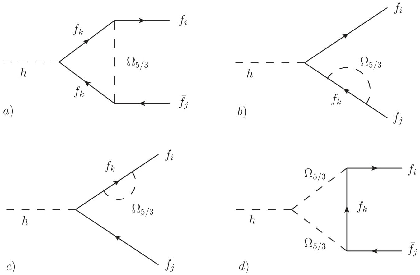
FIGURE 5 Feynman diagrams for the rare decay h  fif-j induced by the scalar leptoquarks. In particular we consider the contribution of the leptoquark with electric charge 5/3 which arises from the leptoquark doublet R 2

Once the invariant amplitude for each Feynman diagram was written down, we used the Passarino-Veltman reduction scheme to solve the loop integrals [67], which was carried out with the implementation of the Mathematica package socalled Package-X [68]. After some algebraic simplifications, the invariant amplitude can be written in the form

M(hτμ)=u¯(pτ)(FLPL+FRPR)v(pμ), (9)

where the F L and F R form factors are given in terms of Passarino-Veltman scalar functions and can be consulted in Appendix B.

After summing over the polarization of the final fermions, we introduce the average squared amplitude into the twobody decay width formula to obtain

Γ(hτμ)=λ1/2(mh2,mμ2,mτ2)16πmh3×(|FL|2+|FR|2pμpτ-2mμmτReFLFR*). (10)

where Γ(hτμ)=Γ(hτ-μ+)+Γ(hτ+μ- and the scalar product is pμpτ=(mh2-[mμ2+mτ2])/2. We write the exact formula for the decay width, which includes the interference term proportional to lepton masses. However, for the numerical calculations, we omit such a term since it is at least four orders of magnitude less than the main contribution.

4.1. Branching ratio BR(hτµ)

Once the free model parameters involved in the decay width were constrained, we are ready to present the BR(hτμ), which is displayed as a function of the LQ model parameters involved in the process. We consider a Higgs boson mass of 125 GeV whose total width is Γ h = 4.07 × 10⁻³ GeV.

Figure 6 shows the contours of
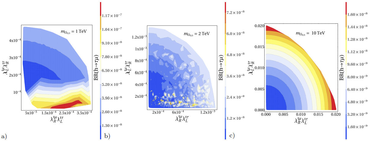
 BR(hτμ) as a function of λL,Rtτ(tμ) couplings in the λRtμλLtτ-λLtμλRtτ plane, for mΩ5/3=1,2,10 TeV.

FIGURE 6 Branching ratio of the decay hτµ as a function of λR(L)tμλL(R)tτ couplings for a) mΩ5/3=1 TeV, b) mΩ5/3=2 TeV, c) mΩ5/3=10 TeV. 

We observe that there are regions in the λRtμλLtτ-λLtμλRtτ plane in which the BR(hτμ), for an LQ mass of mΩ5/3=1 TeV, has values up to 10−7. While in the case of mΩ5/3=10 TeV, a BR(hτμ) of order up to 10−8 is predicted. We note that this small variation in the branching ratio is due to that λR(L)tμλL(R)tτ increases as mΩ5/3 increases, as shown in Fig. 3. We also note that our results are lower by up to 6 orders of magnitude than the result reported by the authors of Ref. [48]. They found a BR(hτμ) of up to 1%, where the destructive cancellation among amplitudes is achievable by fine-tuning. Nevertheless, this encouraging result is now excluded by the upper limit imposed by the ATLAS and CMS [29, 30] collaborations: 0.28%,0.25%, respectively. Similar rates can be found in the Refs. [50, 51] in which an explanation for an apparent excess of the BR(hτμ) reported by the CMS [52] and ATLAS [53] collaborations was provided. The authors of Ref. [69] have analyzed the decay hτµ mediated by the leptoquark with quantum numbers (3,1,-1/3) (corresponding to the leptoquark S 1 in the nomenclature of Ref. [46]). Specifically, they found a BR(hτμ) of order 10−9 and 10−7, assuming a value for λ S of O(1) and O(4π), respectively. These results are comparable with ours, although we are not considering a value for λ so close to the perturbative limit. Furthermore, the phenomenology of the leptoquark S 1 has been studied in Ref. [70], where they found that S 1 can also explain the predicted and measured value of the µAMDM.

4.2. Number of signal events

Let us first explicitly mention the background and signal processes:

  • SIGNAL: We consider the main production mode of the Higgs boson at hadron colliders, i.e., the gluon fusion mechanism with its subsequent decay into a τµ pair:

gghτμeντνeμ. (11)

The electron channel must contain exactly two opposite-charged leptons, namely, one electron and one muon. Therefore, we search for the final state plus missing energy due to undetected neutrinos.

  • BACKGROUND: The potential SM background arises from:

    1. Drell-Yan process, followed by the decay Zττ τ ν e µν τ ν µ .

    2. WW production with subsequent decays W e and Wµν µ .

    3. ZZ production, later decaying into Zττ τ ν e µν τ ν µ and Zνν.

Table I shows the number of background events in which we consider the optimally integrated luminosities associated with each collider, namely: HL-LHC, 3 ab−1; HE-LHC, 12 ab−1; FCC-hh, 30 ab−1. We compute the cross-section of all background processes with MadGraph5 at NLO in QCD [71].

TABLE I Number of background events. In all cases we take into account the optimal integrated luminosities: HL-LHC, 3 ab−1; HELHC, 12 ab−1; FCC-hh, 30 ab−1

Background
process
HL-LHC HE-LHC FCC-hh
Drell-Yan 194988300 1474246800 12337410000
WW production 5031000 50400000 503100000
ZZ production 69720 584400 10161000

As far as the signal is concerned, we present in Fig. 7 the number of signal events produced at the HL-LHC as a function of λR(L)tμλL(R)tτ couplings for mΩ5/3=1,2,10 TeV and an integrated luminosity L=3  ab-1. While in the Figs. 8, 9 are shown the corresponding cases for the HE-LHC and FCC-hh, respectively.

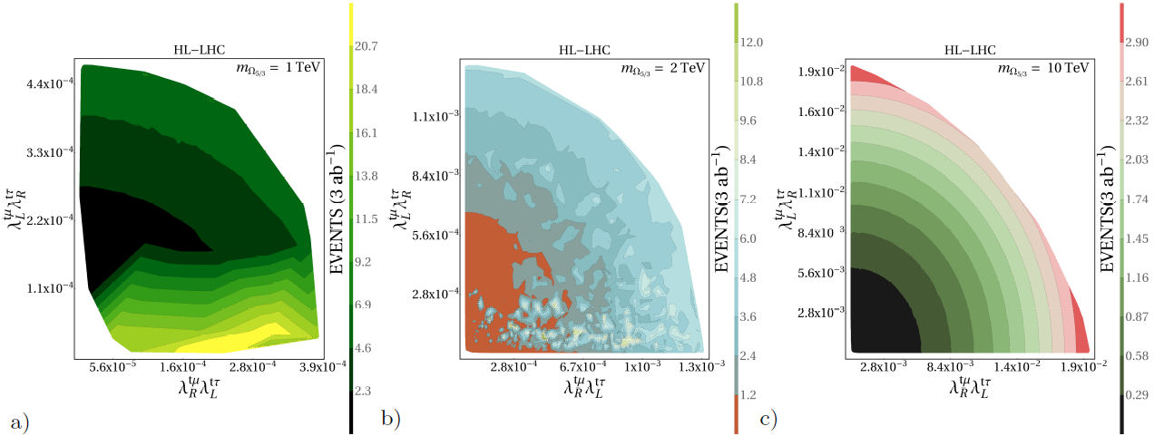
FIGURE 7 Number of signal events produced at the HL-LHC as a function of λR(L)tμλL(R)tτ couplings for a) mΩ5/3=1 TeV, b) mΩ5/3=2 TeV, c) mΩ5/3=10 TeV. In all cases we use L=3  ab-1

FIGURE 8 The same as in Fig. 7 but for the HE-LHC and L=12  ab-1

FIGURE 9 The same as in Fig. 7 but for the FCC-hh and L=30  ab-1

We note that for specific regions in the λRtμλLtτ-λLtμλRtτ plane, the number of signal events for an LQ mass of mΩ5/3=1 TeV could reach about 21 (252, 4230) events at the HL-LHC (HE-LHC, FCC-hh). As far as mΩ5/3=2 TeV is concerned, the number of events produced at the HL-LHC (HE-LHC, FCC-hh) is closer to 12 (150, 2500). Finally, for an LQ mass of mΩ5/3=10 TeV the events produced are 3 (35, 590) at the HL-LHC (HE-LHC, FCC-hh).

Although the branching ratio BR(hτμ) is very suppressed and not detectable in current colliders, we analyzed the feasibility for the study of hτµ decay at future colliders. In order to isolate the signal from the background processes, inspired in the strategies of ATLAS and CMS collaborations [52,72], we applied the kinematic cuts shown in Table II, where we have considered the following benchmark point: λmΩ5/3=1 TeV and s=100 TeV for an integrated luminosity of Lint=30  ab-1, i.e., for the FCC-hh.

TABLE II Kinematic cuts applied to the signal and main SM background for the FCC-hh with a center-of-mass energy s=100 TeV and Lint=30  ab-1 and mΩ5/3=1 TeV. 

Cut number Cut NS NB (≈) SFCC-hh
Initial (no cuts) 4230 1.29 × 10¹⁰ 0.0373145
1 |ηe | < 1.5 3891 4.6 × 10⁹ 0.0572067
2 |ηµ | < 1.5 3780 2.78 × 10⁹ 0.0717467
3 0.1 <R(e, µ) 3671 1.25 × 10⁹ 0.10387
4 40 < pT (e) 3592 1.2 × 10⁸ 0.321392
5 50 < pT (µ) 3422 8.37 × 10⁷ 0.374058
6 40 < MET 3257 1.92 × 10⁷ 0.742309
7 110 < mcol(e, µ) < 140 3081 1.6 × 10⁶ 2.43522
8 25 < MT (e) 2987 1.2 × 10⁶ 2.70744
9 15 < MT (µ) 2879 9.2 × 10⁵ 2.99237

We observe that the main kinematic cut is the collinear mass, which is defined as:

mcoleμ=minveμx,  with  x=|PTe||PTe|+ETmissPTe,  and  minveμ,  and minveµ the visible invariant mass. (12)

5. Conclusions

The decay width of the LFV decay hτµ in the context of a simple LQ model with no proton decay was calculated.

This model incorporates to the SM a SU(2) scalar LQ doublet with hypercharge Y = 7/6. In such a model a non-chiral LQ with electric charge Q = 5/3e that couples to charged leptons and up-type quarks are predicted, which contributes to the LFV decay of the Higgs boson.

As far as the analytical results are concerned, we present them in terms of Passarino-Veltman scalar functions. As for the numerical analysis, in order to have a realistic calculation, we obtained bounds on the parameter space involved in the

calculations via the most up-to-date experimental constraints on the LHC Higgs boson data, the muon and electron (g−2), the LFV radiative decays τµγ and µ, explaining all the processes simultaneously.

We find that for specific regions of the allowed parameter space in the λRtμλLtτ-λLtμλRtτ plane, the BR(hτμ) is of order 10−9 − 10−7. Although these results are highly suppressed, we impose kinematic cuts to isolate the signal as much as possible, and we found that the signature is out of detection in current colliders, but evidence for the hτµ decay could be had at the FCC-hh.

Acknowledgments

M. A. Arroyo-Ureña especially thanks to PROGRAMA DE BECAS POSDOCTORALES DGAPA-UNAM for postdoctoral funding and thankfully acknowledge computer resources, technical advice, and support provided by Laboratorio Nacional de Supercómputo del Sureste de México. This work was supported by projects Programa de Apoyo a Proyectos de Investigación e Innovación Tecnológica (PAPIIT) with registration codes IA106220 and IN115319 in Dirección General de Asuntos de Personal Académico de Universidad Nacional Autónoma de México (DGAPA-UNAM), and Programa Interno de Apoyo para Proyectos de Investigación (PIAPI) with registration code PIAPI2019 in FES-Cuautitlán UNAM and Sistema Nacional de Investigadores (SNI) of the Consejo Nacional de Ciencia y Tecnología (CONACYT) in México.

References

1. G. Aad et al., Observation of a new particle in the search for the Standard Model Higgs boson with the ATLAS detector at the LHC, Phys. Lett. B 716 (2012) 1. https://doi.org/10.1016/j.physletb.2012.08.020. [ Links ]

2. S. Chatrchyan et al., Observation of a New Boson at a Mass of 125 GeV with the CMS Experiment at the LHC, Phys. Lett. B 716 (2012) 30 https://doi.org/10.1016/j.physletb.2012.08.021. [ Links ]

3. G. C. Branco, P. M. Ferreira, L. Lavoura, M. N. Rebelo, M. Sher and J. P. Silva, Theory and phenomenology of two Higgs-doublet models, Phys. Rept. 516 (2012) 1. https://doi.org/10.1016/j.physrep.2012.02.002. [ Links ]

4. J. L. Diaz-Cruz, R. Noriega-Papaqui and A. Rosado, Mass matrix ansatz and lepton flavor violation in the THDM-III, Phys. Rev. D 69 (2004) 095002. https://doi.org/10.1103/PhysRevD.69.095002. [ Links ]

5. J. L. Diaz-Cruz, A More flavored Higgs boson in supersymmetric models, JHEP 05 (2003) 036. https://doi.org/10.1088/1126-6708/2003/05/036. [ Links ]

6. M. A. Arroyo-Ureña, J. L. Diaz-Cruz, E. Díaz and J. A. Orduz-Ducuara, Flavor violating Higgs signals in the Texturized Two-Higgs Doublet Model (THDM-Tx), Chin. Phys. C 40 (2016) 123103-1. https://doi.org/10.1088/1674-1137/40/12/123103. [ Links ]

7. M. A. Arroyo-Ureña, J. L. Díaz-Cruz, G. Tavares-Velasco, A. Bolaños and G. Hernández-Tomé, Searching for lepton flavor violating flavon decays at hadron colliders, Phys. Rev. D 98 (2018) 015008. https://doi.org/10.1103/PhysRevD.98.015008. [ Links ]

8. R. Gaitán, J. H. Montes de Oca and J. A. Orduz-Ducuara, Probing flavor parameters in the scalar sector and new bounds for the fermion sector, PTEP 2017 (2017) 1. https://doi.org/10.1093/ptep/ptx084. [ Links ]

9. Q. R. Ahmad et al., Measurement of the rate of νe + d → p + p + e interactions produced by 8B solar neutrinos at the Sudbury Neutrino Observatory, Phys. Rev. Lett. 87 (2001) 071301-1. https://doi.org/0.1103/PhysRevLett.87.071301. [ Links ]

10. T. Araki et al., Measurement of neutrino oscillation with KamLAND: Evidence of spectral distortion, Phys. Rev. Lett. 94 (2005) 081801. https://doi.org/10.1103/PhysRevLett.94.081801. [ Links ]

11. Q. R. Ahmad et al., Direct evidence for neutrino flavor transformation from neutral current interactions in the Sudbury Neutrino Observatory, Phys. Rev. Lett. 89 (2002) 011301. https://doi.org/10.1103/PhysRevLett.89.011301. [ Links ]

12. K. Eguchi et al., First results from KamLAND: Evidence for reactor anti-neutrino disappearance, Phys. Rev. Lett. 90 (2003) 021802. https://doi.org/10.1103/PhysRevLett.90.021802. [ Links ]

13. Y. Fukuda et al., Evidence for oscillation of atmospheric neutrinos, Phys. Rev. Lett. 81 (1998) 1562. https://doi.org/10.1103/PhysRevLett.81.1562. [ Links ]

14. Y. Ashie et al., Evidence for an oscillatory signature in atmospheric neutrino oscillation, Phys. Rev. Lett. 93 (2004) 101801. https://doi.org/10.1103/PhysRevLett.93.101801. [ Links ]

15. M. H. Ahn et al., Measurement of Neutrino Oscillation by the K2K Experiment, Phys. Rev. D 74 (2006) 072003. https://doi.org/10.1103/PhysRevD.74.072003. [ Links ]

16. Z. Maki, M. Nakagawa and S. Sakata, Remarks on the unified model of elementary particles, Prog. Theor. Phys. 28 (1962) 870. https://doi.org/10.1143/PTP.28.870. [ Links ]

17. A. Pilaftsis, Lepton flavor nonconservation in H0 decays, Phys. Lett. B 285 (1992) 68. https://doi.org/10.1016/0370-2693(92)91301-O. [ Links ]

18. J. G. Korner, A. Pilaftsis and K. Schilcher, Leptonic CP asymmetries in flavor changing H0 decays, Phys. Rev. D 47 (1993) 1080. https://doi.org/10.1103/PhysRevD.47.1080. [ Links ]

19. J. L. Diaz-Cruz and J. J. Toscano, Lepton flavor violating decays of Higgs bosons beyond the standard model, Phys. Rev. D 62 (2000) 116005. https://doi.org/10.1103/PhysRevD.62.116005. [ Links ]

20. T. Han and D. Marfatia, h → µτ at hadron colliders, Phys. Rev. Lett. 86 (2001) 1442. https://doi.org/10.1103/PhysRevLett.86.1442. [ Links ]

21. K. A. Assamagan, A. Deandrea and P. A. Delsart, Search for the lepton flavor violating decay A0 /H 0 → τ±µ at hadron colliders, Phys. Rev. D 67 (2003) 035001. https://doi.org/10.1103/PhysRevD.67.035001. [ Links ]

22. E. Arganda, A. M. Curiel, M. J. Herrero and D. Temes, Lepton flavor violating Higgs boson decays from massive seesaw neutrinos, Phys. Rev. D 71 (2005) 035011. https://doi.org/10.1103/PhysRevD.71.035011. [ Links ]

23. A. Brignole and A. Rossi, Anatomy and phenomenology of mu-tau lepton flavor violation in the MSSM, Nucl. Phys. B 701 (2004) 3. https://doi.org/10.1016/j.nuclphysb.2004.08.037. [ Links ]

24. J. L. Diaz-Cruz, D. K. Ghosh and S. Moretti, Lepton Flavour Violating Heavy Higgs Decays Within the nuMSSM and Their Detection at the LHC, Phys. Lett. B 679 (2009) 376. https://doi.org/10.1016/j.physletb.2009.07.065. [ Links ]

25. A. Lami and P. Roig, H → ll’ in the simplest little Higgs model, Phys. Rev. D 94 (2016) 056001. https://doi.org/10.1103/PhysRevD.94.056001. [ Links ]

26. S. Chamorro-Solano, A. Moyotl and M. A. Pérez, Lepton flavor changing Higgs Boson decays in a Two Higgs Doublet Model with a fourth generation of fermions, J. Phys. G 45 (2018) 075003. https://doi.org/10.1088/1361-6471/aac458. [ Links ]

27. M. A. Arroyo-Ureña, T. A. Valencia-Pérez, R. Gaitán, J. H. Montes De Oca and A. Fernández-Téllez, Flavor-changing decay h → τµ at super hadron colliders, JHEP 08 (2020) 170. https://doi.org/10.1007/JHEP08(2020)170. [ Links ]

28. G. Hernández-Tomé, J. I. Illana and M. Masip, The ρ parameter and H0 → lilj in models with TeV sterile neutrinos, Phys. Rev. D 102 (2020) 113006. https://doi.org/10.1103/PhysRevD.102.113006. [ Links ]

29. A. M. Sirunyan et al. [CMS], Search for lepton flavour violating decays of the Higgs boson to µτ and eτ in proton-proton collisions at √s = 13 TeV, JHEP 06 (2018) 001. https://doi.org/10.1007/JHEP06(2018)001. [ Links ]

30. Searches for lepton-flavour-violating decays of the Higgs boson in √s = 13 TeV pp collisions with the ATLAS detector, ATLAS-CONF (2019) 013. http://cds.cern.ch/record/2674131. [ Links ]

31. G. Apollinari, O. Brüning, T. Nakamoto and L. Rossi, High Luminosity Large Hadron Collider HL-LHC, CERN Yellow Rep. 05 (2015) 1. https://doi.org/10.5170/CERN-2015-005.1. [ Links ]

32. M. Benedikt and F. Zimmermann, Proton Colliders at the Energy Frontier, Nucl. Instrum. Meth. A 907 (2018) 200. https://doi.org/10.1016/j.nima.2018.03.021. [ Links ]

33. N. Arkani-Hamed, T. Han, M. Mangano and L. T. Wang, Physics opportunities of a 100 TeV proton-proton collider, Phys. Rept. 652 (2016) 1. https://doi.org/10.1016/j.physrep.2016.07.004. [ Links ]

34. P. Bandyopadhyay and R. Mandal, Revisiting scalar leptoquark at the LHC, Eur. Phys. J. C 78 (2018) 491. https://doi.org/10.1140/epjc/s10052-018-5959-x. [ Links ]

35. H. Georgi, The State of the Art-Gauge Theories, AIP Conf. Proc. 23 (1975) 575. https://doi.org/10.1063/1.2947450. [ Links ]

36. H. Georgi and S. L. Glashow, Unity of All Elementary Particle Forces, Phys. Rev. Lett. 32 (1974) 438. https://doi.org/10.1103/PhysRevLett.32.438. [ Links ]

37. H. Fritzsch and P. Minkowski, Unified Interactions of Leptons and Hadrons, Annals Phys. 93 (1975) 193. https://doi.org/10.1016/0003-4916(75)90211-0. [ Links ]

38. J. C. Pati and A. Salam, Unified Lepton-Hadron Symmetry and a Gauge Theory of the Basic Interactions, Phys. Rev. D 8 (1973) 1240. https://doi.org/10.1103/PhysRevD.8.1240. [ Links ]

39. J. C. Pati and A. Salam, Lepton Number as the Fourth Color, Phys. Rev. D 10 (1974) 275. https://doi.org/10.1103/PhysRevD.10.275. [ Links ]

40. J. R. Ellis, M. K. Gaillard, D. V. Nanopoulos and P. Sikivie, Can One Tell Technicolor from a Hole in the Ground?, Nucl. Phys. B 182 (1981) 529. https://doi.org/10.1016/0550-3213(81)90133-4. [ Links ]

41. E. Farhi and L. Susskind, Technicolor, Phys. Rept. 74 (1981) 277. https://doi.org/10.1016/0370-1573(81)90173-3. [ Links ]

42. L. J. Hall and M. Suzuki, Explicit R-Parity Breaking in Supersymmetric Models, Nucl. Phys. B 231 (1984) 419. https://doi.org/10.1016/0550-3213(84)90513-3. [ Links ]

43. B. Schrempp and F. Schrempp, LIGHT LEPTOQUARKS, Phys. Lett. B 153 (1985) 101. https://doi.org/10.1016/0370-2693(85)91450-9. [ Links ]

44. W. Buchmuller, Composite Quarks and Leptons, Acta Phys. Austriaca Suppl. 27 (1985) 517. https://doi.org/10.1007/978-3-7091-8830-98. [ Links ]

45. B. Gripaios, Composite Leptoquarks at the LHC, JHEP 02 (2010) 045. https://doi.org/10.1007/JHEP02(2010)045. [ Links ]

46. I. Doršner, S. Fajfer, A. Greljo, J. F. Kamenik and N. Košnik, Physics of leptoquarks in precision experiments and at particle colliders, Phys. Rept. 641 (2016) 1. https://doi.org/10.1016/j.physrep.2016.06.001. [ Links ]

47. J. M. Arnold, B. Fornal and M. B. Wise, Phenomenology of scalar leptoquarks, Phys. Rev. D 88 (2013) 035009. https://doi.org/10.1103/PhysRevD.88.035009. [ Links ]

48. K. Cheung, W. Y. Keung and P. Y. Tseng, Leptoquark induced rare decay amplitudes h → τµ± and τ → µγ, Phys. Rev. D 93 (2016) 015010. https://doi.org/10.1103/PhysRevD.93.015010. [ Links ]

49. A. Bolaños, R. Sánchez-Vélez and G. Tavares-Velasco, Flavor changing neutral current decays t → cX (X = γ, g, Z, H) and t → cll (l = µ, τ) via scalar leptoquarks, Eur. Phys. J. C 79 (2019) 700. https://doi.org/10.1140/epjc/s10052-019-7211-8. [ Links ]

50. I. Doršner, S. Fajfer, A. Greljo, J. F. Kamenik, N. Košnik and I. Nišandžic, New Physics Models Facing Lepton Flavor Violating Higgs Decays at the Percent Level, JHEP 06 (2015) 108. https://doi.org/10.1007/JHEP06(2015)108. [ Links ]

51. S. Baek and K. Nishiwaki, Leptoquark explanation of h → µτ and muon (g − 2), Phys. Rev. D 93 (2016) 015002. https://doi.org/10.1103/PhysRevD.93.015002. [ Links ]

52. V. Khachatryan et al., Search for Lepton-Flavour-Violating Decays of the Higgs Boson, Phys. Lett. B 749 (2015) 337. https://doi.org/10.1016/j.physletb.2015.07.053. [ Links ]

53. G. Aad et al., Search for lepton-flavour-violating H → µτ decays of the Higgs boson with the ATLAS detector, JHEP 11 (2015) 211. https://doi.org/10.1007/JHEP11(2015)211. [ Links ]

54. W. Buchmuller, R. Ruckl and D. Wyler, Leptoquarks in Lepton - Quark Collisions, Phys. Lett. B 191 (1987) 442. https: //doi.org/10.1016/0370-2693(87)90637-X. [ Links ]

55. A. Bolaños, A. Moyotl and G. Tavares-Velasco, Static weak dipole moments of the τ lepton via renormalizable scalar leptoquark interactions, Phys. Rev. D 89 (2014) 055025. https://doi.org/10.1103/PhysRevD.89.055025. [ Links ]

56. M. Aaboud et al., Searches for third-generation scalar leptoquarks in √s = 13 TeV pp collisions with the ATLAS detector, JHEP 06 (2019) 144. https://doi.org/10.1007/JHEP06(2019)144. [ Links ]

57. A. M. Sirunyan et al., Search for heavy neutrinos and third-generation leptoquarks in hadronic states of two τ leptons and two jets in proton-proton collisions at √s = 13 TeV, JHEP 03 (2019) 170. https://doi.org/10.1007/JHEP03(2019)170. [ Links ]

58. A. M. Sirunyan et al., Search for pair production of second-generation leptoquarks at √s = 13 TeV, Phys. Rev. D 99 (2019) 032014. https://doi.org/10.1103/PhysRevD.99.032014. [ Links ]

59. E. Keith and E. Ma, S, T, and leptoquarks at HERA, Phys. Rev. Lett. 79 (1997) 4318. https://doi.org/10.1103/PhysRevLett.79.4318. [ Links ]

60. T. Aoyama et al., The anomalous magnetic moment of the muon in the Standard Model, Phys. Rept. 887 (2020) 1. https://doi.org/10.1016/j.physrep.2020.07.006. [ Links ]

61. G. W. Bennett et al., Final Report of the Muon E821 Anomalous Magnetic Moment Measurement at BNL, Phys. Rev. D 73 (2006) 072003. https://doi.org/10.1103/PhysRevD.73.072003. [ Links ]

62. M. Sorbara, The muon g-2 experiment at FERMILAB, Frascati Phys. Ser. 69 (2019) 170. [ Links ]

63. L. Morel, Z. Yao, P. Cladé and S. Guellati-Khélifa, Determination of the fine-structure constant with an accuracy of 81 parts per trillion, Nature 588 (2020) 61. https://doi.org/10.1038/s41586-020-2964-7. [ Links ]

64. R. H. Parker, C. Yu, W. Zhong, B. Estey and H. Müller, Measurement of the fine-structure constant as a test of the Standard Model, Science 360 (2018) 191. https://doi.org/10.1126/science.aap7706. [ Links ]

65. P. A. Zyla et al., Review of Particle Physics, PTEP 2020 (2020) 083C01. https://doi.org/10.1093/ptep/ptaa104. [ Links ]

66. M. A. Arroyo-Ureña, R. Gaitán and T. A. Valencia-Pérez, SpaceMath version 1.0. A Mathematica package for beyond the standard model parameter space searches, [arXiv:2008.00564 [hep-ph]]. [ Links ]

67. G. Passarino and M. J. G. Veltman, One Loop Corrections for e+ e- Annihilation Into mu+ mu- in the Weinberg Model, Nucl. Phys. B 160 (1979) 151. https://doi.org/10.1016/ 0550-3213(79)90234-7. [ Links ]

68. H. H. Patel, Package-X: A Mathematica package for the analytic calculation of one-loop integrals, Comput. Phys. Commun. 197 (2015) 276. https://doi.org/10.1016/j.cpc.2015.08.017. [ Links ]

69. M. Bauer and M. Neubert, Minimal Leptoquark Explanation for the R D(∗) , RK , and (g − 2)g Anomalies, Phys. Rev. Lett. 116 (2016) 141802. https://doi.org/10.1103/PhysRevLett.116.141802. [ Links ]

70. Y. Cai, J. Gargalionis, M. A. Schmidt and R. R. Volkas, Reconsidering the One Leptoquark solution: flavor anomalies and neutrino mass, JHEP 10 (2017) 047. https://doi.org/10.1007/JHEP10(2017)047. [ Links ]

71. J. Alwall, M. Herquet, F. Maltoni, O. Mattelaer and T. Stelzer, MadGraph 5 : Going Beyond, JHEP 06 (2011) 128. https://doi.org/10.1007/JHEP06(2011)128. [ Links ]

72. G. Aad et al., Search for lepton-flavour-violating decays of the Higgs and Z bosons with the ATLAS detector, Eur. Phys. J. C 77 (2017) 70. https://doi.org/10.1140/epjc/s10052-017-4624-0. [ Links ]

73. R. Benbrik and C. K. Chua, Lepton Flavor Violating l → l’γ and Z → ll’ Decays Induced by Scalar Leptoquarks, Phys. Rev. D 78 (2008) 075025. https://doi.org/10.1103/PhysRevD.78.075025. [ Links ]

Appendix

A. Analytical expressions for the calculation of constraints

A.1 Radiative decay τµγ and µAMDM

For the sake of completeness, we present the exact expressions for the decay f i f j γ induced by the leptoquark Ω 5/3 . Thereby the form factors L and R of Eq. (8) can be written as

L=Ncmi16π2mΩ5/32q=t,c(mjλRqjλRqiαRR+miλLqjλLqiαLL+mqλLqjλRqiαLR), (A.1)

R=L(λLqlλRql), (A.2)

where the explicit form of the coefficients α i is

αRR=QΩk12ηji2-xj(xi-2ξq)+ξqxiΛxj,1,xq/xj+xi-ξqΛxi,1,xq-2ηjiCΩΩq0+ηji2xj2xi2xjxi+ξq2ηjilog(xq)-ηjixjxj-ξq+Qq12ηji2xj(xi+2ξq)-ξqxiΛxj,1,xq/xj-xi+ξqΛxi,1,xq+2xqηjiCqqΩ0+ηji2xj2xi2xqxjxi+ξq2ηjilog(xq)+ηjixjxj+ξq, (A.3)

αLR=QΩk1ηjiΛxj,1,xq,-1ηjiΛxi,1,xq,+ξq2xjxilogxq+Qq1ηjiΛxj,1,xq,-1ηjiΛxi,1,xq,+ξq2xjxilogxq+CqqΩ0, (A.4)

where we employ the shorthand notation xi=mi2/mΩ5/32, ξ i = x i −1 and η ij = x i x j . The function Λ(x 1 ,x 2 ,x 3) is given by

Λ(x1,x2,x3)=λ(x1,x22,x32)2x101dz1x1z+(-x1+x32-x22)z+x32, (A.5)

with λ the triangle function: λ(x1,x2,x3)=x12+x22+x32-2x1x2-2x2x3-2x3x1. We also define the following set of Passarino-Veltman scalar functions:

CΩΩq0=mΩ5/32C0(0,mj2,mi2,mΩ5/32,mΩ5/32,mq2), (A.6)

CqqΩ0=mΩ5/32C0(0,mj2,mi2,mq2,mq2,mΩ5/32). (A.7)

The coefficient α LL can be obtained from α RR by exchanging the external fermion masses.

From the Eqs. (A.3) and (A.4) one can obtain the approximate expressions in the limit of small x i and x j (limit of vanishing external fermion masses). Then the following results are valid for the LFV decay τµγ and the µAMDM

I(xq)=αRR(xq)QΩk1-6xq+3xq2-6xq2logxq12xq-14+Qq-2+3xq-6xq2+xq3+6xqlogxq12xq-14, (A.8)

J(xq)=αLR(xq)QΩk--1+xq2-2xqlogxq21-xq3+Qq3-4xq+xq2+2logxq21-xq3. (A.9)

The above expressions agree with the formulas presented in [73].

B. Form factors F L,R contributing to the hτµ decay

In order to write the form factors F R and F L of Eq. (9), we first define the following set of Passarino-Veltman scalar functions

Δμ=B0mμ2,mΩ5/32,mq2-B00,mΩ5/32,mq2, (B.1)

Δτ=B0(mτ2,mΩ5/32,mq2)-B0(0,mΩ5/32,mq2), (B.2)

Δμτ=B0(mμ2,mΩ5/32,mq2)-B0(mτ2,mΩ5/32,mq2), (B.3)

Δhμ=B0(mh2,mq2,mq2)-B0(mμ2,mΩ5/32,mq2), (B.4)

Δhτ=B0(mh2,mq2,mq2)-B0(mτ2,mΩ5/32,mq2), (B.5)

CqqΩh=mΩ5/32C0(mh2,mμ2,mτ2,mq2,mq2,mΩ5/32), (B.6)

CΩΩqh=mΩ5/32C0(mh2,mμ2,mτ2,mΩ5/32,mΩ5/32,mq2). (B.7)

The form factor F R of Eq. (9) can be written as

FR=Nc16π2(βLLλLqμλLqτ+βRRλRqμλRqτ+βRLλRqμλLqτ+βLRλLqμλRqτ). (B.8)

where the coefficient β LL has the following form

βLL=gmΩ5/3xq2mWxμλ(xh,xμ,xτ)λxh,xμ,xτ2xqημτξqxμΔτ-xτΔμ-xμxτΔμτ-xμημτ-xhημh+2ξq+xτCqqΩh+xhxμ-ξq-xq+ξμημτlog(xq)+2xμ-ηhμ+xτxhΛxh,xq,xq-xμ-ηhτxμΛxμ,1,xq+2xτxτΛxτ,1,xq+λΩvxμmΩ5/3xμλ(xh,xμ,xτ)ημh+xτxμΛxμ,1,xq+xhξq+xτ+xτ-ξqημτCΩΩqh+log(xq)2xμxhξq+xμ-xμ-ξqημτ+xτ-ημHΛxh,1,1-2xτ2Λxτ,1,xq. (B.9)

The coefficient β RR can be obtained from β LL by exchanging the lepton masses: β RR = β LL (m µ m τ ). As for the coefficients β RL and β LR , they have the following form

βRL=gmΩ5/3xq4mWλ(xh,xμ,xτ)2λxh,xμ,xτxτΔhμ-xμΔhτημτ-1+2xτ2xh+ημτΛxτ,1,xq+2xμ2ηhμ+xτ×Λxμ,1,xq-2xhxμ+xτ-ημτ2xhΛxh,xq,xq-2CqqΩhxhηhμ+2xτxμ+3xhxqημτ-xτ+xqxh2+2ημτ2-log(xq)ημτ2-xhxμ+xτ-2ξq-λΩvmΩ5/3xqCΩΩqh, (B.10)

βLR=gmΩ5/3xqxμxτ2mWλ(xh,xμ,xτ)λxh,xμ,xτητμΔμτ-xhηhμ-2ξq-xτCqqΩh-2xhΛxh,xq,xq+xμxh+ημτΛxμ,1,xq+xτxh-ημτΛxτ,1,xq+log(xq)2xμxτ2xμxτxh-ξqxμ+xτxh+ξqημτ2. (B.11)

The form factor F L can be obtained from F R employing the following replacement

FL=FR(λLqlλRql). (B.12)

If we consider the limit of vanishing external fermion masses, Eq. (B.10) reduces to

βRLmq,mΩ53mqvB0mh2,mq2,mq2-B00,mΩ53,mq2+λΩv2C00,mh2,0,mq2,mΩ532,mΩ532+mq2+mΩ532C00,mh2,0,mΩ532,mq2,mq2 (B.13)

and the remaining β i functions vanish in such a limit. This result agrees with the one presented in [48,50].

Received: November 03, 2020; Accepted: January 09, 2021

Creative Commons License This is an open-access article distributed under the terms of the Creative Commons Attribution License