1. Introduction

For centuries, physical theories have influenced various areas of science, including economics. For example, Hetherington states that the efforts of Adam Smith to establish the general laws of economics are motivated by the Newton’s achievement in establishing the fundamental laws of motion ¹. During the last decades, physicists have successfully studied economic systems, giving rise to a new discipline called Econophysics ^{2,3,4,5,6,7,8}.

A simple model of economic exchange was proposed in which money, as energy, is conserved in each interaction, resulting in a wealth distribution identical to the Boltzmann-Gibbs distribution for energy, where the temperature corresponds to the average money or energy of the system ⁹. Based on conserving money, multiple works were carried out in which mechanisms such as savings, taxes and dynamics to support the poorest population were implemented ^10,11,12 yielding distributions which are not longer pure exponentials and tend to decrease wealth inequalities.

Within the spirit of conservative exchanges, here we propose a model with upper bounds that limits the amount of wealth agents can possess. This limit produces a piling up of agents in fewer states causing more ordering of the system or less wealth inequality. When the imposed upper bound is too close to the average wealth, then we will numerically show a transition to systems with negative temperatures. Negative temperatures formally exist in paramagnetic materials exposed to external magnetic fields because mathematically the slope (which is proportional to the temperatures) of the entropy as a function of the total energy is negative. Also, the existence of negative temperatures has been studied in social systems in Axelrod’s social influence model ¹³.

2. Economic Exchange Interaction Model With Upper Bounds

In the study of income and wealth distributions in economics, one of the most used inequality indicators is the Gini index (GI) given by

Here x _i and x _j are the wealth values of agents i and j, respectively, M is the total wealth and N is the number of economic agents. Thus, GI equal to zero expresses perfect equality, where all values are the same (for example, where everyone has the same wealth) and GI = 1 (or 100%) expresses maximal inequality among values (e.g., occuring when only one person has all the wealth, and all others have none).

Since we can safely assume that money is conserved in short periods of time when billions of economic interactions (or steps) amongst agents occur, we use a model which consists of a closed economic system composed of fixed total wealth M and number of economic agents N. To each i-agent is assigned an initial amount of wealth m _i that can be conservatively exchanged with other agents. The iterative interactions are made between two agents i and j selected randomly, which exchange wealth obeying the following expressions:

Here mi' y mj' are the final wealth of agents i and j, respectively, and k is a random value between 0 and 1. Although here we choose N = 3000, it can be shown that such relatively small number yields fortunately the same qualitative results than larger and more realistic economic models. A particular “realization” is defined as a system that follows the rules given by Eq. 2, but two realizations are different because the randomness of the choice of agents and the value of k. This dynamics is exactly the same as that occurring in a physical system of collisions between particles so that depending on how collision occurs, the energy gain or loss of a given particle may be abrupt (if it is near a head-on collision) or very small (if the angle of deflection is large). Therefore, in the economics analogy an agent can become rich or poor in one or many interactions. A savings model ¹⁰, in which the agents gain or lose a fraction of their wealth in each interaction, is a more realistic model of commerce or economic exchanges.

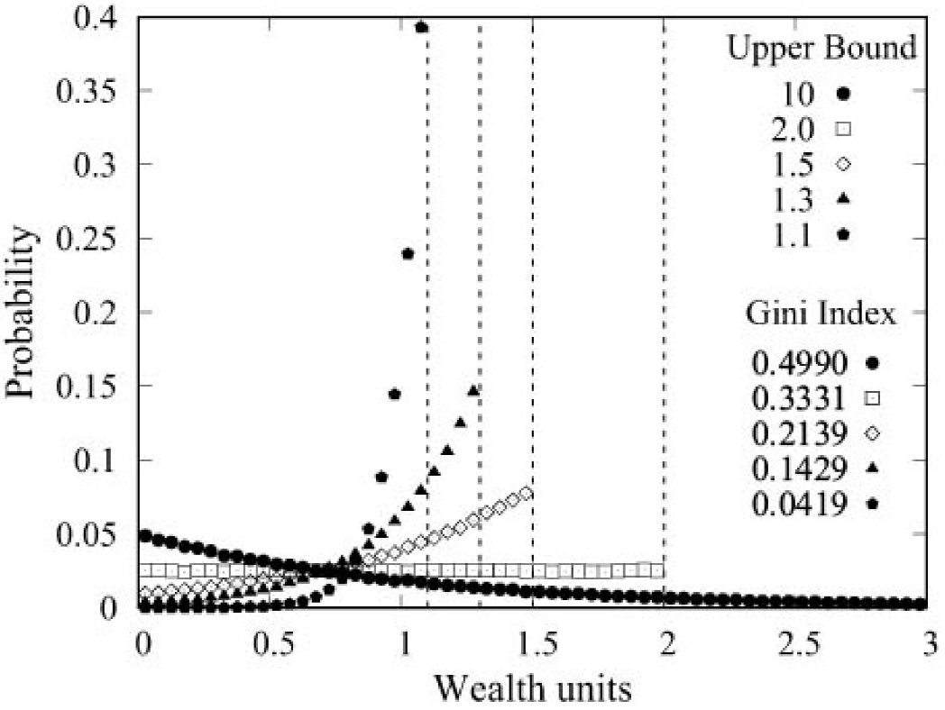
In order to reduce the economic inequality of the system, we establish wealth upper bounds (UB) to forbid the existence of “too rich” agents. That is, economic interactions that result in an agent whose final wealth exceeds an established limit are canceled. We assign an initial wealth of m ₀ = 1 unit to each agent and, therefore, the system average wealth (SAW = M/N) is equal to 1. With these values, we show in Fig. 1 the results of a series of simulations with m ₀ as a wealth unit, UB = 10, 2, 1.5, 1.3 and 1.1, averaging over 30 realizations.

Figure 1. Probability distributions P with different UB values with 3000 agents interacting 3 × 10⁵ times according to Eq. 2 with an initial wealth of 1 unit per agent. The horizontal scale is cut. 

As can be seen, there are no agents beyond the bound because the UB strictly forbids agents to have a wealth greater than the UB; therefore, this barrier reduces inequality as the UB decreases as shown by the GI. Notice how distributions in Fig. 1 change their slope as the UB decreases. When the bound is large (UB = 10), then GI = 0.4990 which is very similar to the value of 0.5 corresponding to the exponential Maxwell-Boltzmann distribution obtained from Eq. 2 without imposing any upper bound; which means that the system is unaffected by an UB set well above the SAW and therefore, the agents can freely increase his wealth according to the random value k. But when UB is too close to SAW then the distribution P becomes very narrow and peaked. It’s important to mention that our results are very robust since they don’t depend on the initial wealth conditions; that is, we could have started with a random distribution of wealth or, in an extreme case, assigning all the wealth to only one agent and the results would be the same.

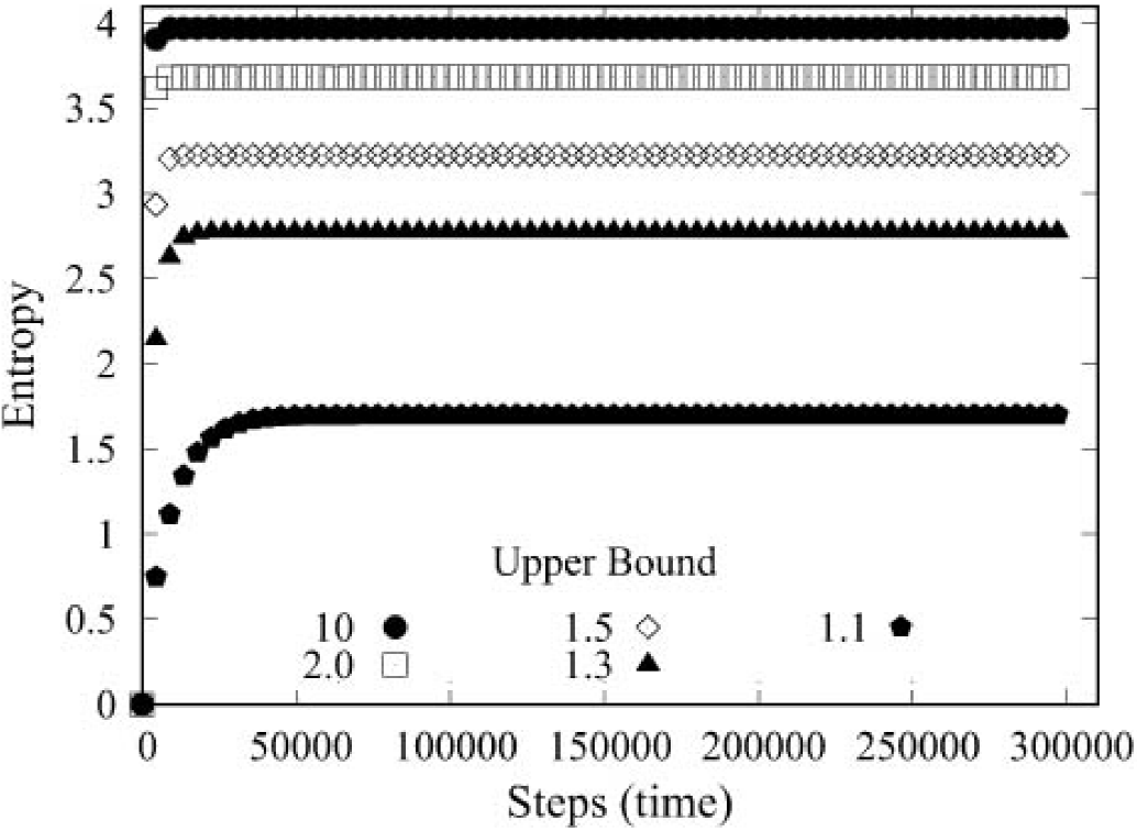
For the same values of UB, the associated time evolution of entropy S = - ΣP(m)ln⁡[Pm] is shown in Fig. 2.

Figure 2. Entropy as a function of time. 

The constant values of S show that distributions are stable. When the UB is lowered, the maximum entropy value decreases taking longer to reach stability. GI and S are tools that analyze the disorder of a given distribution, however, the GI compares the form of the distribution with an equity distribution and determines the amount of relative inequality, while S which arises naturally from physical laws, can also determine whether the system is in equilibrium or not. This ordering phenomenon, characterized by a decrease in entropy, has similarities with the alignment of the magnetic moments of a paramagnetic material subjected to a variable external field studied by Landau mencioned in next section ¹⁴.

3. Paramagnetic Materials and Exchange Model Exhibit Negative Temperatures

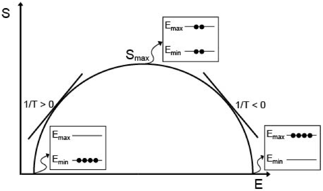
Now we will discuss the appearance of negative temperatures in paramagnetic materials and in our system. A partial alignment of the atomic magnetic moments is observed in paramagnetic materials when they are subjected to external magnetic fields modifying the system energy. As the intensity of the external magnetic field increases, the magnetic moments move to a higher energy levels, increasing the entropy of the system, until reaching the point of maximum entropy. Then, an increase in the system energy causes the moments to begin to settle into the highest energy level (E _max ), because the allowed energy levels are limited. In that case, the entropy decreases because the system is more ordered and its temperature (T = (dS/dE)^-1), which is the inverse of the slope of the entropy curve as a function of energy, is negative, as shown esquematically in Fig. 3.

Figure 3. Schematic plot of Entropy S vs. total Energy E. Only four spins or particles are shown to illustrate some cases of ordering in two levels. 

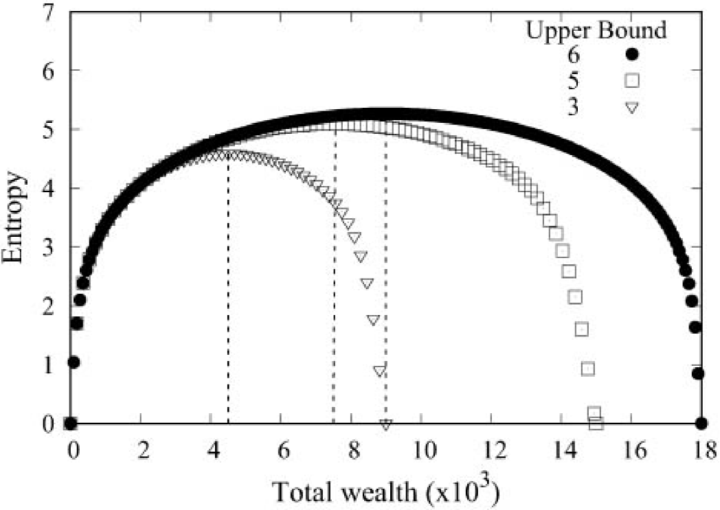
In order to achieve the phenomenon of negative temperatures in our economic case, we make simulations with the same number of agents N = 3000, but with different total wealth and three values of the upper bound (UB = 6, 5 and 3), up to 3 × 10⁵ interactions according to Eq. 2. Figure 4 shows the corresponding results averaged over 30 realizations.

Figure 4. Entropy S for different values of UB as a function of the system total wealth M. Each point represents the average equilibrium entropy of 30 realizations and the lines show the point of maximum entropy in each case. 

Notice that these curves show the same qualitative behavior and are similar to the schematic diagram shown in Fig. 3. When UB is too low then most interactions are not allowed, and in the limit when UB is equal to SAW there is no economic activity in the system, and therefore the system is perfectly ordered and the temperature is zero. According to T = (dS/dM)^-1, Fig. 5 shows the corresponding exotic temperature behavior when UB = 6.

Figure 5. Temperature T as a function of the total wealth M. 

As can be seen, there is a transition in temperature which goes from positive to negative when the system has a wealth of 9 × 10³ units, i.e., when the SAW is equal to 3 units which is half the value of the UB.

4. Discussions

In econophysics, the temperature has been considered as an indicator of system income or wealth, while any inequality index and the entropy of the corresponding distribution yields information on the associated dispersion or broadening. Our simulations clearly show how the entropy S changes as a function of both the total energy and the upper bound value. Entropy measures how much order exist in the system in the sense that more agents with the same energy or wealth represent lower entropy values. In our model, if the upper bound is much greater than the system average wealth, then the richest agents are “less affected" by the limiting condition and can interact more freely, but if the value of the upper bound is lower, then the entropy S and the Gini index GI decrease, indicating an ordering, which is observed as a lower dispersion in distribution. In other words, the upper bound imposes an “impermeable barrier" which prevents agents to go beyond the barrier in the wealth axis. Thinking of money as energy, then negative temperatures exist at the theoretical physics level, as a consequence of the fact that the entropy function with respect to the energy (wealth) of the system becomes decreasing. In our model of economic exchanges that conserve energy, we obtained that lowering the upper bound yields lower Gini index and entropy. In the extreme case that the upper bound is very close to the system average wealth, then the distribution is very peaked and narrow at the expense of forbidding some kind of economic exchanges. Ours is a particular extreme case of how entropy is lowered by imposing strong restrictions on the system to get negative temperatures. In other words, negative temperatures imply more restrictions for exchanges especially for wealthier agents who can not increase their wealth.

These restrictions or limitations of accessible energies in our model remind us Maxwell’s demon that selects those particles that may or may not pass a certain barrier. Our model is not easy to implement in physical systems such as particle gases. However, the economic counterpart is plausible through a strong tax policy aimed at the upper economic sectors. This taxing mechanism prevents the agents from having a wealth greater than a predefined limit. However, since in reality it is not possible to apply such a strict policy, then a permeable upper bound could be modeled which allows some agents to go through the barrier and have greater wealth and to investigate the properties of the final distribution especially at the point of transition to negative temperatures.

We hope that this work may stimulate further research in income or wealth distributions in econophysics and negative temperatures in novel systems.