Introduction

Mexico City is mostly affected by seismic events occurring in the subduction zone of the Cocos plate in Michoacán, Guerrero and Oaxaca states. The hypocenter of the September 19, 1985, occurred at Michoacán coast at (17.6 N y 102.5 W) with a magnitude M_w of 8.1 (IGFIIN, 1985), at a depth of 15 km (^{USGS, 1985}) and inflicted an enormous damage in the city. Cities within 150 km from Mexico City and at similar distances to the Middle America Trench (MAT) have never been so strongly affected by large magnitude seismic events. Puebla and Toluca, neighboring, populated state capitals, did not report the type of damage experienced by the nation’s capital in the above and other strong earthquakes. This indicates that Mexico City possesses certain characteristics that are peculiar of its geographic location that seem to enhance seismic events. One peculiarity of the Mexico basin is indeed the existence of an ancestral lake that filled the basin in which Mexico City has been expanding since the XIVth century. Although this lake has been progressively fragmented and desiccated there still remain many areas with saturated sediments. Building in these areas has traditionally required particular civil engineering expertise. ^{Bribiesca (1960)} presented various stages of the lake evolution, illustrating how the lake’s surface has changed over time. Although surface water has evaporated or drained out of the basin, subsurface water still saturate many portions of the upper clay formations. Based on surface geology three regions of different geological characteristics have been traditionally defined (^{Marsal and Mazari, 1969}) for the Mexico City area: hills, transition, and lake deposits. This classification corresponds to geologic formations not deeper than 300 m. A description of the deeper characteristics of the basin is still missing. This work aims at describing them at depths reaching 3 km in the region encompassing the length of the basin in the E-W direction and from Sierra del Tepeyac to Xochimilco in the N-S direction.

Geologic description

The basin of Mexico contains numerous volcanic edifices in and around its limits. Their ages range from Mid Tertiary to Pliocene and Pleistocene. Mid Tertiary deposits are found in Sierra del Tepeyac and the Xochitepec range SW of the basin, and outcrops are present at the footsteps of the ranges E and W of the basin. In the Pliocene, Sierra del Tepeyac flows were reactivated ejecting considerable amounts of dacitic and rhyolitic lavas. In the Upper Pliocene the north drainage of the basin was blocked by flows of basaltic andesite. Erosion of the ranges confining the basin produced alluvial fans that filled the canyons until the Lower Pleistocene (^{Marsal and Mazari, 1969}). A new episode of volcanic activity started in the Pleistocene following SW to NE fractures in the crust covering the region with layers of basalt and pumice. Several volcanic structures belong to this episode (Chiconautla, Chimalhuacán and Cerro de la Estrella). Discharge of the basin was towards the south at this time, until the basin’s drainage was blocked again by the emplacement of Sierra Chichinautzin in the Upper Quaternary, and a lake developed in its interior. As previously mentioned, this ancestral lake was subsequently fragmented into several lakes within the basin. The lake corresponding to the location of Mexico City has been drained and embanked since colonization by the Aztecs. Initially embankments or “Calzadas” were built on the lake, subsequently expanding, reaching a point in the last stages such that only water channels persisted as water bodies. Eventually, even those channels were filled out; however, the underlying formations remained saturated. The only remaining channels in the region are those found in the southern Xochimilco Lake.

An objective of this study is revealing the basement topography of Mexico City’s basin. Basement here means the boundary between higher-density formations and sediments. Some of the models to be described ahead show a peculiar pattern for the density distribution in the basin. They show higher densities towards the surface in many locations underlain by low-density materials. One would expect the reverse distribution; a tentative explanation for this phenomenon is that profuse distribution of dense volcanic materials, such as volcanoes and lava flows, have been emplaced on top of the calcareous formations and sedimentary fill throughout the basin. A case in point is that of Ciudad Universitaria where basaltic rocks of ~20m-thickness overlie low-density tuffs and volcanic breccias extending down to 1580 m depth (^{CENAPRED, 1996}). Since lakes and lake deposits are also present in the surface, surface patterns may be observed between the two media in which higher density materials alternate with the lower-density layers. Empirical relations between seismic wave speed and density have been developed (^{Gardner et al., 1974}; ^{Brocher, 2005}); generally, low densities correspond to low velocities and high densities to high velocities.

Previous models

^{Marsal and Mazari (1969)} made reference to the unpublished report of the geophysical contractor that performed the gravimetric measurements (Figure 1). Assuming an Earth’s crust with only two components for the main strata with densities of 1.8 and 2.6 g/cm³, the former corresponding to alluvial and lacustrine deposits, and the latter to igneous masses, they reached the conclusion that the maximum depression in the basin reaches about 1000 m. However, they didn’t point at the location, or locations, where this occurs, recommending additional seismic exploration and borings in order to make more precise determinations.

The model of ^{Álvarez (1988)} appears to be the only previous attempt in describing the basement structure in the western portion of Mexico basin in a quantitative fashion. Using the same data reported above, sampled in a mesh of 225 points, complemented with a bicubicspline interpolation (^{González-Casanova and Álvarez, 1985}), it develops a gravity mesh that was subsequently used to perform 3-D forward modeling of the gravimetric field observed. The final model consists of a dozen rightrectangular prisms that represent basement outcrops (three prisms) and buried structures with a distribution of densities of 2.75 g/cm³ for the denser materials and sediment layers in the 2.27-2.52 g/cm³ range. The prism distribution is N-S extending from Sierra del Tepeyac to Cerro de la Estrella. Towards the W the prisms descend en échelon in 200-m steps reaching a depth of 1000 m. This model corresponds to the area in which the largest damage was recorded in the September 19, 1985, earthquake in Mexico City.

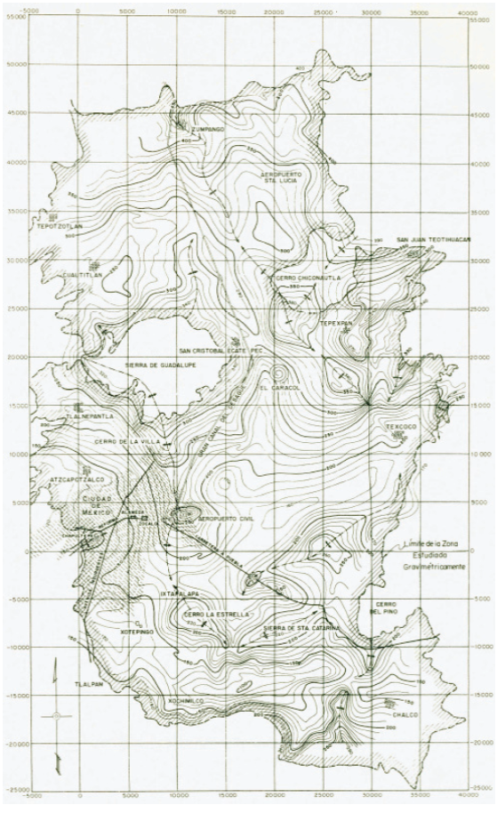
Figure 1 The gravimetric map reported by ^{Marsal and Mazari, (1969)}. Contour values divided by 10 are mGals. Rectangular coordinates are in meters. 

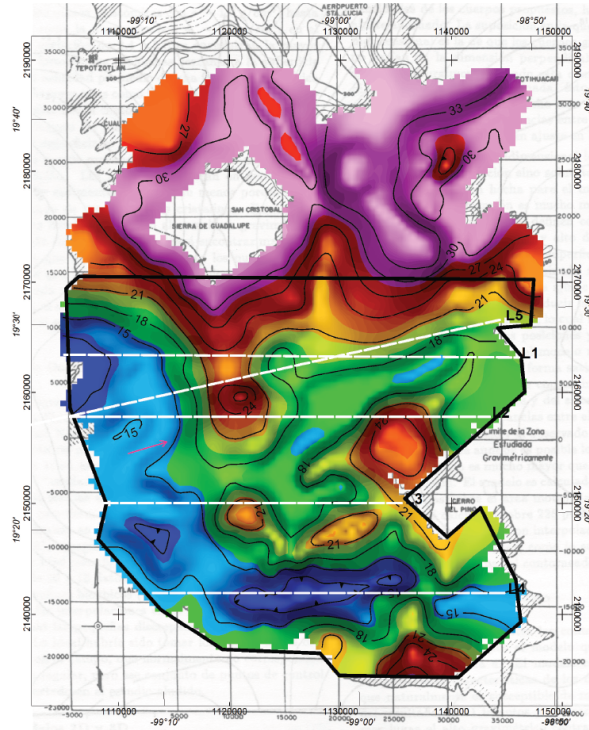
Figure 2a Gravimetric map resampled and contoured from that in Figure 1. Contour values are in mGals. Coordinates are geographic and UTM. The reference polygon (black) for the 3-D inversion is included, as well as five dashed lines (L1 to L5) indicating the location of the gravity models discussed in the text. 

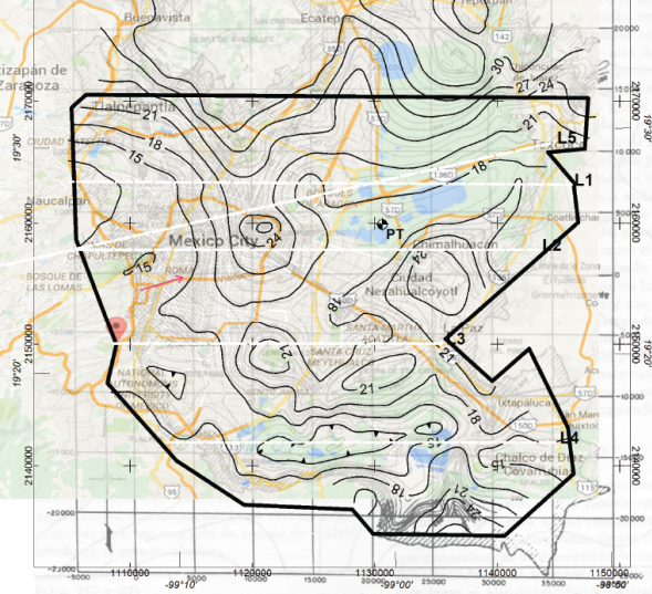
Figure 2b The contours of the Bouguer anomaly are superposed to a reference map in which various locations in the study area can be identified. The reference polygon and L1 to L5 are the same as in Figure 2a. PT approximate location of Pozo Texcoco (^{Marsal and Graue, 1969}) that penetrated 2065 m. 

Gravity inversión

Various new approaches to 3-D potential field inversion are now available (e.g., ^{Camacho et al. 2002}; ^{Montesinos et al. 2003}), which appeared after the forward model reported by ^{Álvarez (1986 b)} for a portion of the basin of Mexico. They are being applied more frequently to the modeling of volcanic edifices, including their magma chambers (^{Represas et al., 2012}; ^{Álvarez and Yutsis 2015}). In the present case the inversion method described by ^{Macleod and Ellis (2013)} was used, based in turn in the theoretical considerations of ^{Ellis et al. (2012)}. A 3-D mesh is built under a selected surface area in which a grid of magnetic or gravity values is defined. In the present case the selected surface area is delimited by the polygon in Figure 2a. Each volume element (voxel) of the mesh is assigned a density or a magnetic susceptibility value, depending on the type of inversion performed. Next, the contribution to the total field of each voxel is calculated at an observation point in the surface. The total contribution of the set of voxels is compared to the corresponding measured value on the surface. The process is repeated for each observation point in the surface until the difference between the calculated and measured values is less than a predetermined value. In the present case this value was chosen to be 5 percent of the standard deviation. Thus the grid generated by the inversion process does not differ from the measured grid more than 5 percent of the standard deviation. In the present inversions grid dimensions within the polygon are 43 x 37 x 8 cells of X=1.0, Y=1.0, and Z= 0.5 km respectively. Padding cells are added where appropriate, to fulfill computation requirements.

Modeling is performed on the gravimetric field only, since aeromagnetic data over this region are missing (^{NAMAG, 2002}). 3-D inversion of the gravity field yielded the density distribution in Figure 3a, showing the inverted volume clipped along L4 and the full (unclipped) density range. Darker colors correspond to higher densities and lower ones to lower densities. Notice the presence of a narrow SW-NE surface alignment of higher density materials (volcanic) across practically all the inverted region; it apparently corresponds to the volcanic activity that started in the Pleistocene following SW-NE fractures. Figure 3b shows the inverted volume clipped along azimuth 53° following the above surface alignment; the highest density shown in the vertical section corresponds to the roots of Cerro de la Estrella. Both figures exhibit low-density materials (blue tones) in the deeper layers; these may correspond to Lower Cretaceous limestones that exist in this region below elevations ~1000 m (^{SGM, 2002}), or to mixtures of sedimentary and igneous formations whose densities are averaged in the voxel volumes of 1 x 1 x 0.5 km.

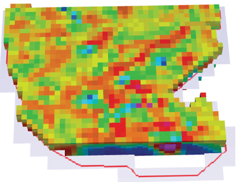
Figure 3a 3-D density distribution obtained from the inversion of the gravity field in Figure 2a. The polygon defining the inverted region is shown in red. The full density range is shown (2.55-2.78 g/cm³). The distribution is clipped along the Y-axis coinciding with L4 Xochimilco-Chalco (see Figure 8). Towards the center, notice the highdensity SW-NE (red) alignment crossing the region almost completely. The depth range is -2750<z<2620 m. 

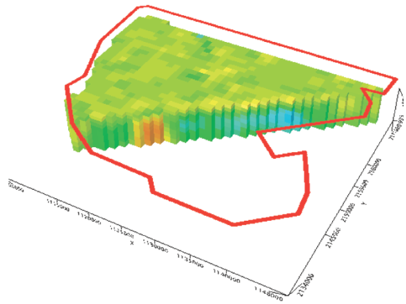
Figure 3b 3-D density distribution obtained from the inversion of the gravity field in Figure 2a clipped along azimuth 53°, along the high-density alignment mentioned in Figure 3a. The full density range is displayed. This view shows a low-density region under Texcoco Lake overlain by the shallow, higher-density materials that form the surface alignment. The depth range is the same as in Figure 3a. Coordinates are UTM. 

The density distribution can now be analyzed selecting density ranges of interest. In Figures 4a through 4f results are presented in various density ranges. The inversion results in the region enclosed by the black polygon in Figure 2a will be analyzed by means of a density clipping process. This way one can select density ranges of interest and see their 3-D distributions under the basin. Figure 4a shows a 3-D rendering of the density volumes in the 2.70-2.78 g/cm³ density range under the basin; all other density values are suppressed. This density range corresponds to the highest densities in the inverted distribution, including the higher density materials outcropping in various places: basalts and dacites. The topography (^{Ryan et al., 2009}) is included for reference purposes. Notably, on the western side of the basin there is a lack of these materials while the eastern side is heavily populated with them. In terms of seismic waves travelling W to E this implies intersecting a density interface where these waves can be reflected back to the west. As mentioned above, ^{Álvarez (1988)} proposed the existence of a canyon in this region, which by now should be filled out with clastic and sedimentary materials.

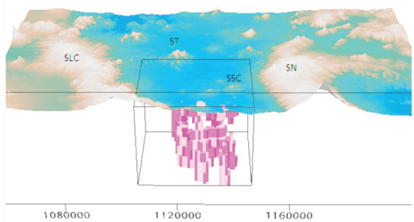
Figure 4a 3-D rendering of the basin of Mexico showing the inverted region in the reference box, displaying the density distribution in the 2.70-2.78 g/cm³ range. The west portion is devoid of these density materials. Vertical exaggeration of 10 gives the rendering an elongated appearance. Topography from ^{Ryan et al. (2009)}. SLC Sierra de Las Cruces, ST Sierra del Tepeyac, SSC Sierra de Santa Catarina, SN Sierra Nevada. 

The distribution of materials within the intermediate density range (2.68-2.74 g/cm³), shows they are intermixed with the higher density materials in the east side (Figure 4b). Materials of intermediate densities begin to populate the west side of the inverted volume.

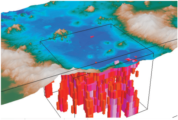
Figure 4b 3-D display of the density distribution in the 2.68-2.74g/cm³ range view from the SW. Magenta represents the lowest values. Vertical exaggeration is 10. Owing to their size, a few voxels pierce the surface of the digital elevation model. 

Intermixed with the above materials there are regions in the next density range (2.572.70 g/cm³) as shown in Figure 4c. Towards the west the region corresponding to the canyon proposed by ^{Álvarez (1988)}, found empty in the high-density range, now appears as an isolated volume. This may represent the canyon filled up with sediments.

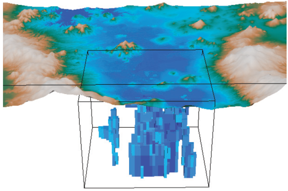
Figure 4c 3-D display of the density distribution in the 2.57-2.70 g/cm³ range. Darker blue corresponds to the lowest densities; notice how on the eastern side they extend to the deepest layers. In the west side appear layers of materials filling out the region previously devoid of high-density materials. Vertical exaggeration is 10. 

In Figure 4d, a perpendicular view, an attempt is made for mapping the regions with lowest densities (2.57-2.63 g/cm³) that should correspond with the water saturated sediments. The correlation of these regions with the presently known saturated zones is quite satisfactory.

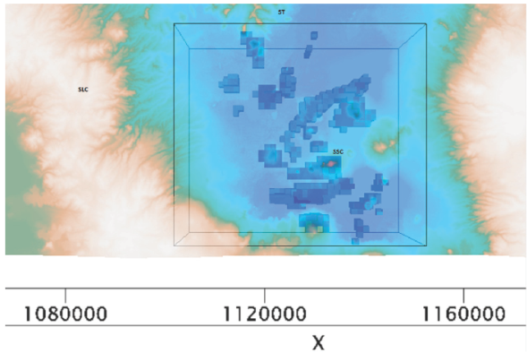
Figure 4d The density distribution in the lowest range (2.57-2.63 g/cm³) is shown in a vertical view. Notice the coincidence between this voxel distribution and the presently mapped regions of saturated lacustrine regions in the basin. 

The view in Figure 4d no7d is changed to view from the south in Figure 4e, which shows that the same density distribution is vertically divided into an upper and a lower cluster, which could not be appreciated in the previous view. The former corresponds to the surface saturated sediments, while the latter is tentatively assigned to Cretaceous limestone formations.

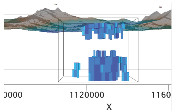
Figure 4e This is the same density distribution as that of Figure 4d, the only change is the orientation of the 3-D view, which is now from the south. It shows two voxel distributions separated by a gap. The upper distribution corresponds to the saturated sediments distribution while the lower one corresponds to a mix of igneous and sedimentary materials. 

A cross-section along the Xochimilco-Chalco region is derived from the inversion, and presented in Figure 4f; it is simply a different way of showing the inversion results, where the blocky voxel appearance has been substituted by an interpolation. It shows high-density materials overlying a low-density distribution. Here we can readily appreciate the link between higher densities and volcanic materials, since at the center we have a volcanic structure (Volcán Xico) and under it a high-density distribution. At about half the depth shown there is a sharp interface separating the high-density region from the lower density distribution, probably corresponding to Cretaceous limestone. The 2-D modeling presented below will complement this result.

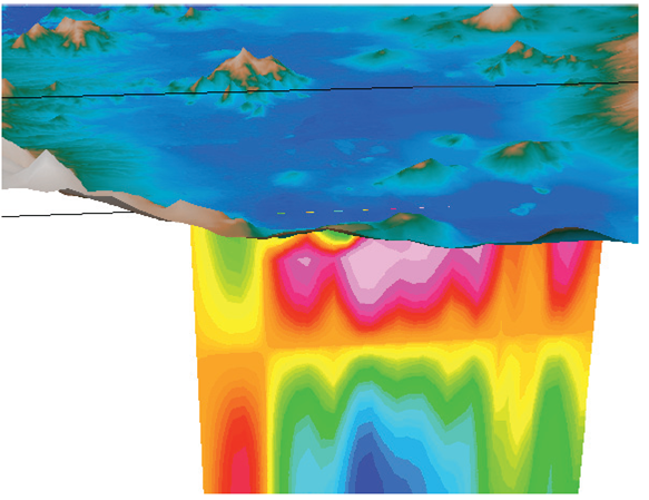
Figure 4f Cross-section along L4 derived from the 3-D inversion. Vertical exaggeration is 10. The blocky appearance in Figures 3a and 3b are substituted by a smooth interpolation. High densities are associated with surface volcanic structures. Deeper low-density regions appear to correspond to limestone formations. 

2-D gravity models

The area analyzed includes all the southern portion of the basin, from Sierra del Tepeyac to the Xochimilco-Chalco region. Five 2-D models are constructed across the basin. Four W-E lines are shown in Figure 2a labeled L1 through L4, and one diagonal (SW-NE) labeled L5. Notice they are contained within the extent of the 3-D inverted area; they are calculated with the ^{Talwani et al., (1959)} algorithm. In the 2-D model, formations above the densest one (basement) consist of layers of lesser densities. Density layers with D=2.55 g/cm³ appear to correspond to lava flows and other volcanic materials, while those with D=2.45 g/ cm³ correspond to clastic Quaternary fill and lake deposits.

L1 runs from Atzcapotzalco to Texcoco (Figure 5). At x= 14 km a positive Bouguer anomaly reflects the presence of the south extension of Sierra del Tepeyac which is buried by sediments. The 2.8 g/cm³ density region shows a steep angle to the west; this density interface is proposed to be a reflector of seismic waves arriving from the west-southwest. In the eastern portion another volcanic region is intercepted at x= 39 km that apparently corresponds to an underground extension of Chimalhuache volcano edifice. The 18 mGal contour in Figure 2a shows a SW-NE elongation around this volcanic structure suggesting that the original intrusion has such an orientation; the NE portion of L1 intercepts this anomaly at that location.

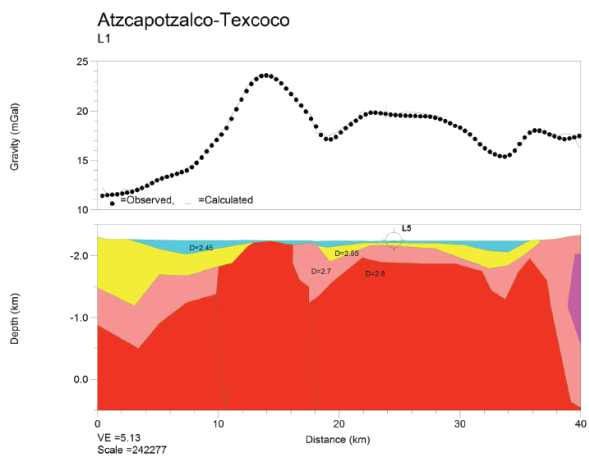
Figure 5 2-D gravity model along L1 to a depth of 500 meters below sea level (mbsl). W is to the left and E to the right. Position marked L5 shows the intersection with that line. The eastern section apparently corresponds with an extension of the anomaly corresponding to Chimalhuache volcano (see Figure 6). 

L2 runs from Bosques in the hills area to Texcoco in the eastern portion of the basin (Figure 6). The west end of this line matches the model of L5, as it should, since both start approximately in the same region, the 2.55 g/ cm³ formation surface in the hills area in both models. Some layers in the 2.70<D<2.75 g/cm³ density range are interpreted as Cretaceous limestones, although the actual nature of these layers cannot be confirmed with this gravity model alone. At x=29 km the line intersects an isolated, dome-type structure above an otherwise flat region. The 2-D model reflects the underground geometry of this formation as a volcanic chimney mapped as andesite (^{SGM, 2002}) corresponding to the monogenetic Chimalhuache volcano. A similar dense structure approach the surface at x= 14 km; it corresponds to the same volcanic formation as Sierra del Tepeyac and Peñón de los Baños.

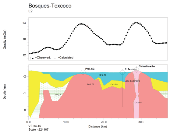
Figure 6 2-D gravity model along L2 to a depth of 500 mbsl. Topography reflects the hills region to the W and the presence of Chimalhuache volcanic structure at x=29 km whose chimney is neatly defined in the model. The body at x=14 km approaching the surface corresponds to the underground extension of Sierra de Guadalupe (Prol. SG). Pozo Texcoco reached 2065 m depth. 

The structure at x=14 km is close to the surface but does not outcrop; however, it outcrops 5 km south of that position, close to the International Airport, at Peñón de los Baños location. Incidentally, this name makes reference to the presence of Temazcales or baths of thermal waters that were used since the Aztec times with medicinal purposes. The presence of these hot springs is intimately linked to recent volcanic activity, confirming its volcanic origin. A geological cross-section inferred across two neighboring exploration wells was reported (^{Marsal and Mazari, 1969}; ^{Álvarez, 1988}) in which the interface between sedimentary/clastic-andesite/basalt reaches 120 m below the surface in that region, providing an additional validation of this model. One well intersected andesites from 220 m to its bottom at 1250 m, and the second well intersected basalts from 500 m to its bottom at 1350 m depth.

Pozo Texcoco (^{Marsal and Graue, 1969}) penetrated 2,065 m (Figure 2b). The stratigraphic column shows conglomerates, breccias, sandstones, sandy-clays, clays, lacustrine limestone, anhydrite, igneous rocks, sandy tuffs, tuffs, ashes and clayey tuffs. The presence of 13 interspersed igneous flows of thicknesses varying from 3.5 to 108 m at depths from 600 to 2000 m denotes great volcanic activity in the Tertiary. In the 3-D inversion the varying densities of these materials are averaged in each voxel of 1 x 1 x 0.5 km dimensions; consequently they may only reflect rough density patterns at their corresponding positions.

L3 runs from Xotepingo to La Caldera in the east (Figure 7). Topography along the line is rather flat except where it intersects two volcanic structures. At x=12 km the volcanic structure intersected corresponds to Cerro de la Estrella, and at x=25 km the volcanic structure appears to be connected with La Caldera volcanic edifice; two volcanic conduits are modeled at those places. A graben-type structure at x=21.5 km, near La Caldera, appears to be presently filled up with volcanoclastic materials. Although aligned with the Sierra del Tepeyac-Peñón de Los Baños structure, Cerro de La Estrella does not belong to it; further ahead (Figure 10a) it will become apparent that they are geologic formations independent of each other, emplaced at different times in the Mexico basin.

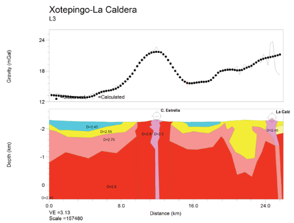
Figure 7 2-D gravity model along L3 to a depth of 500 mbsl. W is to the left and E to the right.Two volcanic structures are intersected: Cerro de La Estrella at x=12 km and La Caldera at x=25 km. The model admits two volcanic chimneys at those places. 

L4 runs W-E from the Tlalpan region to Chalco (Figure 8). The whole region is located within the largest negative Bouguer anomaly and the whole region was covered by a lake until a few decades ago. Actually, that was one of the individual lakes left after the ancestral lake fragmentation. At x=1.8 and x=24.7 km two structures are intercepted in the 2-D model. The former shows only a slight surface deformation and the latter correspond to Xico volcano, which is located 2 km to the north and projected onto L4. The 2-D model and the associated cross-section from the 3-D inversion (Figure 4d) show a remarkable region of low densities towards the center of the line, 15 km in width, starting at a depth of ~1 km and continuing below sea level, and in the case of the cross-section high-density materials associated with volcanic flows overlie the low-density region. The 2-D model, however, shows low-density materials at the top. This discrepancy will be discussed below.

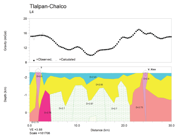
Figure 8 2-D gravity model along L4 to a depth of 500 mbsl. W is to the left and E to the right.The region of low densities toward the center probably corresponds to Cretaceous limestone, mapped under nearby Sierra del Chichinautzin at similar depths (^{SGM, 2002}). 

As reported above, in the Pleistocene the basin contained deep canyons that drained toward the south, prior to the Upper Quaternary emplacement of Sierra del Chichinautzin. It is plausible that the low-density anomaly under discussion corresponds to Creatceous limestone. The presence of higher density materials on top of the sediments can be explained as the result of younger volcanic materials such as lava flows and intrusions populating that region. The limestones would be located between 9<x<16 km with the deepest portion between 12 and 14 km. At x=27 km another low-density region appears at depths below ~1 km. It is possible that this may also correspond to limestones. In a geological cross-section of Sierra del Chichinautzin (^{SGM, 2002}) limestones are present at depths ~1500 m below the surface; this formation also outcrops in neighboring Morelos State.

The model reveals a volcanic chimney that corresponds to Xico volcano located at x=24.5 km that actually fed the volcano. In fact this observation exemplifies how intrusions in this area deposit higher-density materials in the surface, as detected in the inversion process. The cross-section also shows the presence of the volcanic conduit at this position in the form of a thin, medium-density region.

The surface density distributions of the 2-D model and the cross-section from the 3-D model show discrepancies, particularly regarding the uppermost layers. The 2-D model shows lowdensity materials associated with the water saturated layers, while the inverted crosssection shows high-density materials in those layers. The difference arises in the modeling procedure. In the case of the inversion the uppermost layer is defined by voxels of 1 x 1 x 0.5 km in which the densities of the various geologic formations are necessarily averaged. It is apparent that in such volumes the densities of the volcanic materials prevail over those of the sedimentary layers. In the 2-D direct models the averaging process does not exist, although there the assumption is made that the formations extend to infinity in the Y-direction. In spite of these modeling differences there are remarkable coincidences between the results of both procedures, which tend to strengthen the validity of the models, particularly regarding the presence of volcanic structures.

In order to sample the Texcoco Lake region a diagonal line (L5) runs SW to NE (Figure 9); it starts at approximately the same location as L2 (here named Chapultepec), ending north of L1. It also intersects a dense formation (D=2.8 g/ cm³) between 16<x<23 km, interpreted as the underground extension of Sierra del Tepeyac. The Bouguer anomaly of this formation, in a rather flat terrain, reveals the presence of a dense body at that position. The boundaries of this body to the west and east are almost vertical walls; it was probably intruded in the same time span corresponding to the formation of Sierra del Tepeyac. Comparing the western portion of this model with that of L2 one finds neat similarities. The region of Texcoco Lake is located on the eastern half. Under the surface, the model shows the third layer with a density of 2.75 g/cm³ that may represent a mixture of limestone, igneous formations and sedimentary fill.

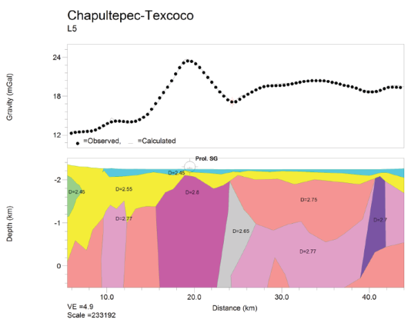
Figure 9 2-D gravity model along L5 to a depth of 500 mbsl. The topography is rather flat except to the west, in the hills region. The mark at x=19 km shows the center of the Sierra de Guadalupe extension (Prol. SG). The Texcoco Lake region is located between 24<x<40 km, where the third layer has a density of 2.75 g/cm³; this layer may represent a limestone formation. 

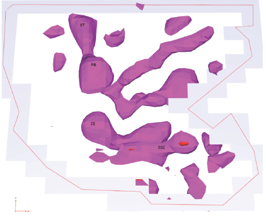
Figure 10a Plan view of the isosurface representing the region where the density has a value of 2.70 g/cm³ in the studied area of the basin of Mexico. This is obtained from the density distribution of the inverted gravity field. The polygon shows the inverted region, as in previous figures. In the south portion, corresponding to Sierra de Santa Catarina (SSC), two red spots pierce the surface, corresponding to higher-density formations enclosed by this surface. ST Sierra del Tepeyac, PB Peñón de Los Baños, CE Cerro de La Estrella. 

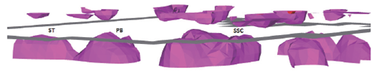
Figure 10b Horizontal view of the surface depicted in Figure 10a from the SW; the dark lines correspond to the representation of the polygon under this projection. A gap devoid of high-density regions is observed between the upper and lower distributions. ST Sierra del Tepeyac, PB Peñón de Los Baños, SSC Sierra de Santa Catarina. 

Discussion

The aim of this study was to try to define regions within the basin of Mexico that may be reflecting surfaces to incoming seismic waves. After reaching such surfaces, an incoming seismic wave would be reflected and refracted.

The possibility of having reflected waves in this region opens the possibility of interaction of these waves with incoming ones. As previously noted, a model of interaction between such waves was proposed (^{Álvarez, 1986a}) that affects the surface saturated layers in such a way as to produce strong, local, vertical motions of the ground, affecting distances of only a few meters, capable of deflecting, and in some cases breaking, tram rails in the vertical direction. It is of the outmost importance to bear in mind the great wavelength difference between these interactions and those of the seismic travelling waves; the former involves meters while the latter involves kilometers.

Using seismic reflection techniques ^{Marsal and Graue (1969}) report seismic wave propagation velocities in the Texcoco Lake area starting with a surface layer of 30 m thickness and 600 m/s velocity. From that depth to ~350 m they found a 1700 m/s layer that ends at “Refractor A” interface, followed by a layer of 2900 m/s ending at another “Refractor B” interface at 1000 m depth. The deepest region showed a 4500 m/s velocity down to the maximum depth of the well (2065 m). The propagation velocity increasing with depth in the formations sampled by the well, appear to be due only to compaction and, consequently, with density increments with depth. Velocities in dense, igneous masses should reach ~6000 m/s. Interaction of arriving and reflected waves should occur in the surface of the low-velocity surface layer, in order to induce the observed damage (^{Álvarez, 1986a}).

Seismic wave reflection may occur at surfaces where there is a density contrast between the geological formations involved (i.e, where a change in propagation velocity occurs). Figure 10a shows a vertical view of the surface in the basin of Mexico where density has a value of 2.70 g/cm³. This surface encloses the volumes in which density is higher than the above value, as can be seen in the south portion of the figure, where two red spots of higher density pierce the surface. Notice that surfaces along the N-S direction will preferentially reflect seismic waves arriving from the W, such as Sierra del Tepeyac, while those along the W-E direction, such as Sierra de Santa Catarina, will preferentially reflect waves from the S. Naturally, reflection phenomena will depend on the magnitude of the earthquake; the higher the magnitude the larger the amplitude of the reflected waves and the larger their effects on the surface.

Figure 10b shows a horizontal view of the same surface, seen from the SW; that is, from the approximate direction of the incoming seismic waves of the September 19, 1985, earthquake. Arriving waves from the hypocenter may have encountered these surfaces, experiencing reflections on them. To the NW, two bodies represent Sierra del Tepeyac formation, separated by what appears to be a gorge covered by sediments. This figure shows a gap between the lower and upper distribution of denser bodies. The upper distribution corresponds to young volcanic edifices and flows covering the basin, while the lower one corresponds to intrusive of older ages associated with the larger surface edifices such as Sierra del Tepeyac and Sierra de Santa Catarina. What appears as a gap in this figure is actually filled with sedimentary materials of lower densities. A similar gap was found in Figure 4e.

Conclusions

The previous model of the deeper geologic formations in the Mexico basin has been extended to include the E-W limits of the basin from Sierra de Las Cruces to Sierra Nevada and from N to S from Sierra del Tepeyac to Sierra del Chichinautzin. The presence of young, dense, bodies on, or close, to the surface was modeled and explained as recent volcanic edifices, usually of the monogenetic type, as well as their flows. The boundaries of the higher-density formations have been defined to depths of ~1 km below sea level suggesting that they are potential reflectors of seismic waves. The former model of ^{Álvarez (1986b)} that proposed the continuity of dense formations between Sierra del Tepeyac to Cerro de La Estrella is now modified, establishing such continuity only up to Peñón de Los Baños since a surface discontinuity is now shown to exist between Peñón de Los Baños and Cerro de La Estrella.

Depending on the orientation of these boundaries they will preferentially reflect seismic waves that are perpendicular to their orientation. It is concluded that waves arriving from the W-SW (e.g., the Michoacán subduction region) will be preferentially reflected by the structure associated with Sierra del TepeyacPeñón de Los Baños, and that seismic waves originating S of the basin (e.g., the GuerreroOaxaca subduction region) will be reflected by Sierra de Santa Catarina, given its E-W extension. ^{Sánchez-Sesma et al., (1988)} made a similar observation suggesting that the latter region could be particularly vulnerable to seismic events originating in southern Mexico.

In Mexico City the region of maximum damage in the September 19, 1985, earthquake was located W of Sierra del Tepeyac-Peñón de Los Baños (e.g., ^{Álvarez, 1986a}, ¹⁹⁹⁰), a region in which saturated sediments and reflecting surfaces coexist, in agreement with the observations made above. The Xochimilco area to the south sustained a comparatively small damage, in spite of being a region where saturated sediments coexist with some of the lakes, but where reflecting surfaces perpendicular to the incoming seismic waves are small or missing.

In order to further test these hypotheses seismic models should be constructed considering the orientation of the incoming seismic waves and the location of the potentially reflecting boundaries described in here.