Article

 

CO₂ flux from the volcanic lake of El Chichón (Mexico)

 

A. Mazot* and Y. Taran

 

Instituto de Geofísica, Universidad Nacional Autónoma de México, Del. Coyoacán, 04510 México City, México E–mail: taran@geofisica.unam.mx * Corresponding author: amazot@geofisica.unam.mx

 

Received: July 1, 2008
Accepted: September 19, 2008

 

Resumen

El flujo de dióxido de carbono fue medido en marzo de 2007 en la superficie del lago del Volcán El Chichón, México, usando el método de la cámara de acumulación flotante. Los resultados de 162 medidas y la aplicación del método estadístico estándar, desarrollado para estos estudios, demuestran que la tasa de emisión total de CO₂ del lago cratérico es relativamente alta. La tasa de emisión total calculada con simulación secuencial Gaussiana fue de 164 ± 9.5 t.d^–1 para el área de superficie del lago de 138, 000 m².

Se proponen dos mecanismos diferentes de desgasificación (por difusión a través de la interfase agua–aire y por burbujas) después de usar el método estadístico gráfico (GSA). Los flujos más altos fueron observados a lo largo de trazas de fallas deducidas. Una desgasificación alta también fue observada a lo largo de lineamentos que concuerdan con fallas que afectan el basamento de la región. Si se considera que el flujo promedio de CO₂ comprendiera todo el fondo del cráter (308,000 m²) se tendría una emisión total del cráter del Volcán El Chichón de por lo menos 370 t.d^–1. Este flujo sería cinco veces más alto que el del lago volcánico de Kelud, Indonesia y similar al flujo de CO₂ de otros volcanes activos con desgasificación pasiva en el mundo.

Palabras clave: Flujo de CO₂, cámara de acumulación, lagos cratéricos, El Chichón.

 

Abstract

Carbon dioxide flux was measured in March 2007 at the surface of the volcanic lake of El Chichón volcano, Mexico using the floating accumulation chamber method. The results of 162 measurements and the application of a standard statistical approach developed for these studies showed that the total CO₂ flux from the crater lake is relatively high. The total emission rate calculated by sequential Gaussian simulation was 164 ± 9.5 t.d^–1from the 138,000 m² area of the lake. Two different mechanisms of degassing (diffusion through the water–air interface and bubbling) are well resolved by a graphical statistical approach (GSA). The highest fluxes were observed along inferred fault traces. Elevated degassing was also observed along main basement faults in the area. The average flux of CO₂ over the entire crater floor of El Chichón (~ 308,000 m²) is inferred to exceed 370 t.d^–1. Thus the total emission rate of CO₂ from El Chichón crater is five times higher than at Kelud volcanic lake, Indonesia, but is similar to emission rates from other passively degassing active volcanoes worldwide.

Key words: CO₂ flux, accumulation chamber, crater lakes, El Chichón.

 

Introduction

Geochemical monitoring of active volcanoes generally includes a periodical or continuous study of the chemistry and/or fluxes of fluids released from the volcano crater or from the volcano edifice where active hydrothermal manifestations are present. In addition to spectroscopic remote sensing of volcanic plumes and direct sampling of fumaroles and hot springs, measurements of the soil diffuse CO₂ degassing by using the method of "accumulation chamber" has become a standard monitoring tool in volcanic and geothermal environments over the last 20 years (e.g. Chiodini et al., 1998). Temporal variations in CO₂ fluxes can be related to changes in the volcanic activity and may be important for the mitigation of the volcanic risk (Hernández et al., 2001a, Notsu et al., 2005). Fluxes of volcanic CO₂ by diffuse degassing through crater floors (Koepenick et al., 1996) or volcanic flanks can be comparable with plume degassing (Wardell et al., 2001). Volcanic craters occupied by a lake include Ruapehu in New Zealand, Poas in Costa Rica, Santa Ana in El Salvador, Kelud in Indonesia and El Chichón in Mexico. In order to measure the gas flux from crater lakes it is necessary to measure fluxes at the water lake surface. Degassing through the lake surface occurs by bubbles (convective/advective degassing) or by diffusion through the water/air interface. Early measurements of diffuse degassing from lakes by using the "floating accumulation chamber" method were made by Kling et al. (1991) for studying biogenic CO₂ production from an Arctic lake. Bernard et al. (2004) and Mazot (2005) were the first to use this method in a volcanic lake (Santa Ana in El Salvador and Kelud in Indonesia).

In this work, we report the first data on CO₂ flux from the surface of the crater lake of El Chichón volcano, Mexico, obtained in March 2007. The aims of this work were (1) to quantify the total CO₂ output from the volcanic lake and the whole crater, (2) to discriminate between mechanisms of degassing (diffusive or by bubbling); (3) to build a CO₂ flux map of degassing patterns from the lake bottom and relate them to local tectonics.

Finally, the total emission rate of CO₂ from El Chichón volcano is compared with those from other volcanic sites.

 

General setting

The El Chichón dome complex (17.36N, 93.23W; 1,100 m.a.s.l.) is located in the northwestern part of the State of Chiapas in southeastern Mexico and halfway between the southeastern end of the Trans–Mexican Volcanic Belt (TMVB) and the northwestern end of the Central American Volcanic Arc (CAVA) (Fig. 1A). Prior to the 1982 eruption, the volcanic structure consisted of two nested andesitic lava domes (maximum elevation of 1260 m a.s.l.) inside a somma crater (Macías et al, 2003; Layer et al., this issue). The 1982 eruption of El Chichón volcano ejected 1.1 km³ of anhydrite–bearing trachyandesite pyroclastic material to form a new 1–km–wide and 200–m–deep crater (Rose et al., 1984). Currently, intense hydrothermal activity, consisting of fumaroles (mainly at the boiling point), steaming grounds, a soap–pool and an acidic (pH≈2.3) and warm lake (~30 °C) occur in the summit crater (Fig. 1B; Taran et al., 1998). With the low pH of the lake, CO₂ is mainly present as a gaseous phase and dissolved in water. So, at this range of pH, the other carbonate species HCO₃– and CO₃²– are not present in the water for which we were sure to measure the whole CO₂ emitted from the lake.

El Chichón lies within an area of folded Jurassic evaporates, Cretaceous limestones, and Tertiary terrigenous rocks (Canul and Rocha, 1981; Duffield et al., 1984). The region is affected by two faults systems oriented approximately N–S and E–W. The most significant fault of the latter system is the San Juan Fault (Fig. 2). Furthermore, the area is characterized by a series of N45° E faults (Chapultenango Fault System) on top of which El Chichón has been emplaced (García–Palomo et al., 2004).

 

Procedure and method

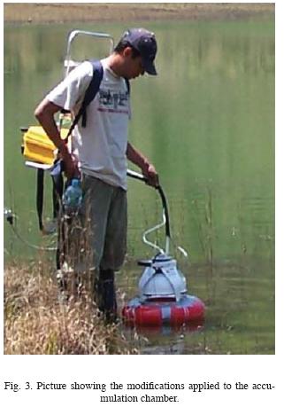
In March 2007, a total of 162 randomly distributed CO₂ flux measurements, covering an area of 138,000 m² of the lake surface, were carried out (Fig. 1B). The GPS position of each measurement point represents the average of two readings (resolution ± 6 m) taken before and after each CO₂ flux measurement (duration 40–60 sec). The drift between these two readings depended greatly on the wind and could attain 40 m. The accumulation chamber method (Chiodini et al., 1998) was modified in order to work on a lake by using a floating chamber (Fig. 3). Gas flux was measured by using a chamber equipped with a LICOR LI–8100–103 infrared CO₂ analyzer (IRGA). The measurement accuracy of the CO₂ flux measurements method is assumed to be ~12.5% (Evans et al., 2001). As the original method from Chiodini et al. (1998), the CO₂ gas coming from the water lake passes through the chamber and the infra–red sensor, it returns to the chamber where it accumulates with the new CO₂ entering the chamber. The flux is derived by obtaining the increase of the CO₂ concentration with time (ppmvol.s^–1). Each measurement takes about 40 to 60 seconds. In order to convert volumetric concentrations to mass concentrations (g.m^–2.d^–1), atmospheric pressure, temperature and total volume (sum of the chamber, IRGA connection tube, and the floating device) were taken in account. The fieldwork was undertaken under dry and stable meteorological conditions.

Computation of total CO₂ flux was based on the graphical statistical approach (GSA) procedure (Chiodini et al., 1998, 2001; Cardellini et al., 2003). This procedure also permits to differentiate the degassing mechanisms of CO₂. GSA consists in the partition of CO₂ flux data into different lognormal populations (using the so–called "inflection" points) and in the estimation of the proportion, the mean and the standard deviation of each population following the graphical procedure of Sinclair (1974). The CO₂ output associated to each population is obtained by multiplying the area of the lake by the proportion and the mean CO₂ flux. The total CO₂ release from the entire studied area can be obtained by summing the contribution of each population. The 90% confidence interval of the mean is used to calculate the uncertainty of the total CO₂ output estimation of each population.

The mapping of degassing areas and estimation of the total CO₂ discharge from the lake and the uncertainty of this estimation, were performed by using the sequential Gaussian simulation (sGs) that is an interpolation algorithm (Deutsch and Journel, 1998). The basic idea of the sGs is to generate a set of equiprobable representations of the spatial distribution of the simulated values, reproducing the statistical (histogram) and spatial (variogram) characteristics of the original data. According to Goovaerts (2001), the differences among all simulated maps (from 100 to 500 realizations) are used to compute the uncertainty of the flux estimation. The sGs approach has already successfully been used for soil CO₂ degassing at other volcanic systems e.g. Chiodini et al., 2007 and details about the method in Cardellini et al., 2003.

 

Results and discussion

Probability distribution of the CO₂flux data

Fig. 4a shows the histogram of log F_CO2 (where F_CO2 is CO₂ flux in g.m^–2.d^–1) versus its frequency. The distribution of CO₂ flux differs from a log–normal distribution indicating that there are at least two different mechanisms of degassing through the lake surface. According to the GSA approach (Sinclair, 1974), the histogram must be transferred to a log probability plot (Fig. 4b). This plot indicates that the CO₂ flux data are separated into two different populations recognizable by the inflection point on the curve corresponding to the 83 cumulative percentile. On the plot we can individuate a high CO₂ population (A in fig. 4b) corresponding to the 17 % of the data and a low CO₂ population (B in fig. 4b) corresponding to the 83 % of F_CO2. The two–population percentages must be checked and validated by combining both populations in the proportion of 17% A and 83 % B at various levels of log F_CO2. The checking procedure uses the following relationship: P_M = f_AP_A + f_BP_B, where P_M is the probability of the "mixture", P_A and P_B are cumulative probabilities of population A and B from the plot of Fig. 4b at a specified x value; f_A and f_B are the proportions of populations A and B. In fig. 4b, the points of the "mixture" are represented by gray triangles. Afterwards, parameters of the individual partitioned populations can be estimated. To estimate the arithmetic mean value of CO₂ flux and the central 90% confidence interval of the mean in the original data units (in g.m^–2.d^–1) for each population, we used, according to Chiodini et al. (1998), the Sichel's t estimator (David, 1977).

A summary of the estimated parameters of partitioned distributions (populations A and B) is reported in Table 1. Population Ais characterized by a mean of 6,702 g.m^–2.d^–1 with a 90% confidence interval of 5,154–10,429 g.m^–2.d^–1. Population B is characterized by a mean of 464 g.m^–2.d^–1 with a 90% confidence interval of 442–490 g.m^–2.d^–1. We suggest that population A corresponds to the flux resulting from bubbles rising through the lake and population B represents the CO₂ degassing by diffusion through the water–air interface (see paragraph 4.3 for details).

The total flow rate of CO₂ released by the lake, calculated by the GSA method, is (6,702 g.m^–2.d^–1 x 0.17% + 464 g.m^–2.d^–1 x 0.83%) x 138,000 m² = 210 t.d^–1with a 90% confidence interval of 172–301 t.d^–1.

Mapping and sgs estimation of the CO₂ flux from the lake

Another statistical method for the estimation of the CO₂ fluxes and the total flow rate is the sequential Gaussian simulation (sGs) (Deutsch and Journel, 1998) method. The 162 measured CO₂ fluxes in randomly distributed points on the lake surface were interpolated by a distribution over a grid of 5,523 square cells (5x5 m²) covering an area of 138,075 m² using the so–called exponential variogram model. Then, 100 simulations of the CO₂ fluxes with the obtained distribution were performed. For each simulation, the CO₂ flux estimated at each cell is multiplied by 25 m² and added to the other CO₂ fluxes estimated at the neighborhood cells of the grid to obtain a total lake CO₂ output. The mean of the 100 total simulated CO₂ outputs, 164 t.d^–1, represents the estimation of the total CO₂ output from the lake area with a standard deviation of 9.5 t.d^–1. The total CO₂ output determined using GSA method is higher (210 t.d^–1) than the mean simulated by the sGs method (164 t.d^–1). In the calculation of the mean of F_CO2, GSA approach does not take into account the spatial correlation between the data, resulting generally in an overestimation of the uncertainty.

The obtained map (Fig. 5) shows that the highest CO₂ flux "spots" are located close to the eastern shore of the lake near the active fumarolic area. Two linear zones of high flux can be clearly recognized on the map, together with several intensively bubbling "funnels" observed during the campaign. These arrangements along NNW–SSE and W–E alignments may be correlated to the regional faults and the E–W San Juan Fault, respectively (García–Palomo et al., 2004).

Estimation of the CO₂ diffusion through the lake–air interface

Our suggestion that the population of data with lower CO₂ fluxes is provided by the diffusion of CO₂ through water–air interface can be checked using the thin boundary layer model (Liss and Slater, 1974). The flux F between water and air may be calculated by the empirical equation (e.g. McGillis and Wanninkhof, 2006):

where k_CO2 is the gas exchange coefficient (in cm.h^–1) for CO₂, C_w and C_w/a , refers to the concentration of CO₂ in water, and in water film at the water–air interface, respectively.

The value of k_CO2 was calculated by using the relationship between windspeed and k_CO2 derived from tracer techniques studies on a small lake (Crusius and Wanninkhof, 2003):

where u₁ is the windspeed measured at 1 m height and Sc is defined as the kinematic viscosity of water at measured temperature divided by the diffusivity of the gas at that temperature. Transfer velocity was adjusted to a Schmidt number of 600 that corresponds to the value for the dissolved atmospheric CO₂ in fresh water at 20°C. The value of Sc_CO2 at 30°C was calculated according to Wanninkhof (1992):

At a mean windspeed u1 of 2 m.s^–1, Sc_CO2 = 360 and k =1.39.

At saturation conditions of 30 °C and 1 atmosphere, C_w of the CO₂ gas is 1.32 mg.cm^–3 (Eq. 1). The concentration of CO₂ in the air–water (C_w/a) interface can be approximated to the concentration of CO₂ in the air–saturated water and corresponds to C≈_w/a10^–5 mg.cm^–3 and C_w>>C_w/a. From the equation (1) and with values for k_CO2 of 1.39 and C_w of 1.32 mg.cm^–3 we estimated a CO₂ flux by diffusion of 442 g.m^–2.d–1 that is very close to the mean value of F_CO2 (464 gm^–2d^–1) for the low flux of data points (population B).

Estimation of the heat power and comparison with other volcanoes in the world

The area of the whole crater floor corresponding to the isohypse 900 m (Fig. 1b) was estimated to be as 308,000 m². Hypothesizing that mains NNW–SSE and W–E alignments are recognized on the lake and that there are not so important variations in F_CO2 in soil and water due to the low depth of the lake (average depth 3 meters see Taran and Rouwet, 2008), a rough estimate of the total CO₂ output for the whole crater floor yields ~370 t.d^–1.

The high CO₂ fluxes plotted on figure 6, show that high CO₂ degassing is not necessarily related to active volcanoes. Three different sources of CO₂ degassing are likely: (1) CO₂, directly coming from a magma chamber, escapes to the surface with other magmatic gases such as SO₂, H₂S, HCl and HF, as this is the case for volcanoes Masaya, Nicaragua (Pérez et al., 2000), Miyakejima and Usu, Japan (Hernández et al., 2001a,b), Stromboli, Italy (Carapezza and Federico, 2000), San Salvador, El Salvador (Pérez et al., 2004), Santa Ana, El Salvador (Bernard et al., 2004) and Galeras, Colombia (Williams–Jones et al., 2000). (2) CO₂ coming from a magma chamber but with a possible contamination due to the crustal carbonate decomposition and subsequent CO₂ release. This type of the CO₂ release could be the case for Solfatara and Vesuvio, Italy (Cardellini et al., 2003; Frondini et al., 2004), Santorini and Nisyros, Greece (Chiodini et al., 1998; Cardellini et al., 2003), Yellowstone, USA (Werner et al., 2000) and Kelud, Indonesia (Mazot, 2005). (3) CO₂ degassing at low temperature and coming from carbonate metamorphism, not related to magmatism. Sites that released this kind of CO₂ are for example Dixie Valley, USA (Bergfeld et al., 2001) and central Italy (Rogie et al., 2000).

The total CO₂ output from El Chichon crater is 1.5 times higher than the effusion rates reported for the summit area at Stromboli (mean flux: 246 t.d^–1; area: 357,500 m²; Carapezza and Federico, 2000) and little lower than those reported for the soil CO₂ flux at Mammoth Mountain in Long Valley Caldera, USA (mean flux: 411 t.d¹; area: 420,000 m²; Sorey et al., 1998).

The CO₂ degassing from the volcanic lake of El Chichón was compared (Fig. 6) with that of Kelud crater lake (Indonesia) and Santa Ana crater lake (El Salvador). In the Kelud crater lake, where CO₂ flux measurements has been carried out since 2001 (Mazot, 2005), the total CO₂ output ranges from 100 t.d^–1 with a mean of 1020 g.m^–2.d^–1 (2001) to 35 t.d^–1 with a mean of 335 g.m^–2.d^–1 (2006) and a constant area of 103,600 m². In Santa Ana, where measurement was performed in 2002, CO₂ output corresponds to 7 t.d^–1 in 2002 with a mean of CO₂ flux of 220 g.m^–2.d^–1 and an area of 30,000 m² (Bernard et al, 2004). Among these three volcanic lakes, the total CO₂ output at El Chichón in 2007 was up to 5 times higher (164 t.d^–1) than Kelud volcano and 23 times higher than Santa Ana (Fig.4).

Fumarolic gas of El Chichón volcano contains about 90 wt% of H₂O (steam) and 10 wt% of CO₂ (Taran et al., 1998; Tassi et al., 2003). Assuming that all the CO₂ released from the crater floor is the result of separation of these gases caused by shallow condensation of hydrothermal steam at ~ 100 °C, beneath the crater floor of the volcano we have ~ 3,700 t/day or ~ 43 kg/s of steam flux and beneath the lake we have ~ 1,640 t/day or ~ 19 kg/s. Using a value for steam enthalpy at 100 °C due to steam condensation (~ 2.257 MJ/kg) we can estimate the heat power due to fumarolic output from the crater floor as 100 and from the lake 43 MW. This heat output is up to 3.5 times higher than the output estimated by Taran and Rouwet (2008) using the heat and chemical balance approach at El Chichón lake. Our estimation based on the direct measurements of fluxes seems to be more realistic.

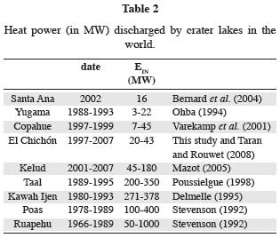
The heat output corresponding to El Chichón lake (43 MW) is comparable with the heat power of other crater lakes of active volcanoes. In Kelud lake, Mazot (2005) calculated values of heat power ranging from 45 to 180 MW in the period 2004–2007 (Table 2) by using the heat and chemical balance model of Stevenson (1992). The heat power was estimated on other crater lakes as Kawah Ijen (Indonesia; Delmelle, 1995), Taal (Philippines; Poussielgue, 1998), Poas (Costa Rica; Stevenson, 1992), Yugama (Japan; Ohba et al., 1994), Ruapehu (New Zealand; Stevenson, 1992) and Copahue (Argentina; Varekamp et al., 2001). The heat output of 100 MW from El Chichón crater is relatively small in comparison with the heat power observed at hot (>40 °C) crater lakes, where values as high as several hundred MW were estimated (Table 2).

 

Conclusion

CO₂ flux measurements made by using the floating accumulation chamber method allowed to estimate the total CO₂ emission from the crater lake of El Chichón (138,000 m²) to be close to 164 t.d^–1. For the total area of the crater floor of 308,000 m² the total CO₂ emission was estimated at 370 t.d^–1. This level of the total CO₂ emission and the estimated heat output are comparable with other volcanic and geothermal areas worldwide.

Continuous monitoring of CO₂ flux from the crater lake of El Chichón could improve our understanding of the hydrothermal system. This would be complementary to other geochemical investigations and it would be particularly important for detecting possible changes in the activity of the volcano.

 

Bibliography

Baubron, J. C., P. Allard, J. C. Sabroux, D. Tedesco and J. P. Toutain, 1990. Soil gas emanations as precursory indicators of volcanic eruptions, J. Geol. Soc. London, 148, 571–576.        [ Links ]

Bergfeld, D., F. Goff and C. J. Janik, 2001. Elevated carbon dioxide flux at the Dixie Valley geothermal field, Nevada; relations between surface phenomena and the geothermal reservoir. Chem. Geol., 177, 43–66.        [ Links ]

Bernard, A., C. D. Escobar, A. Mazot and R. E. Gutiérrez, 2004. The acid volcanic lake of Santa Ana volcano, El Salvador. GSA Special Paper, 375, 121–134.        [ Links ]

Canul, R. F. and V. L. Rocha, 1981. Informe geológico de la zona geotérmica de "El Chichonal," Chiapas: Comisión Federal de Electricidad, Informe (Unpublished internal report).        [ Links ]

Capaccioni, B., Y. Taran, F. Tassi, O. Vaselli, F. Mangani and J. L. Macías, 2004. Source conditions and degradation processes of light hydrocarbons in volcanic gases: an example from El Chichón volcano (Chiapas State, Mexico). Chem. Geol., 206, 81–96.        [ Links ]

Carapezza, M. L and C. Federico, 2000. The contribution of fluid geochemistry to the volcano monitoring of Stromboli. J. Volcanol. Geotherm. Res., 95, 227–245.        [ Links ]

Cardellini, C., G. Chiodini and F. Frondini, 2003. Application of stochastic simulation to CO₂ flux from soil: mapping and quantification of gas release. J. Geophys. Res. 108, 2425, doi:10.1029/ 2002JB002165.        [ Links ]

Chiodini, G., R. Avino, T. Brombach, S. Caliro, C.Cardellini, S. De Vita, F. Frondini, D. Granirei, E. Marotta and G. Ventura, 2004. Fumarolic and diffuse soil degassing west of Mount Epomeo, Ischia, Italy. J. Volcanol. Geotherm. Res., 133, 291–309.        [ Links ]

Chiodini, G., R. Cioni, M. Guidi, B. Raco and L. Marini, 1998. Soil CO₂ flux measurements in volcanic and geothermal areas. Appl. Geochem., 13, 5, 543–552.        [ Links ]

Chiodini, G., F. Frondini, C. Cardellini, D. Granieri, L. Marini and G. Ventura, 2001. CO₂ degassing and energy release at Solfatara volcano, Campi Flegrei, Italy. J. Geophys. Res. 106, B8, 16, 213–16, 221.        [ Links ]

Chiodini, G., A. Baldini, F. Barberi, M. L. Carapezza, C. Cardellini, F. Frondini, D. Granieri, and M. Ranaldi, 2007. Carbon dioxide degassing at Latera caldera (Italy): Evidence of geothermal reservoir and evaluation of its potential energy. J. Geophys. Res., 112, B12204, doi:10.1029/2006JB004896.        [ Links ]

Crusius, J. and R. Wanninkhof, 2003. Gas transfer velocities measured at low wind speed over a lake. Limnol. Oceanogr., 48, 1010–1017.        [ Links ]

David, M., 1977. Geostatistical ore reserve estimation (Developments in geomathematics 2). Elsevier, New–York, 363 pp.        [ Links ]

Delmelle, P., 1995. Geochemical, isotopic and heat budget study of two volcano hosted hydrothermal systems: the acid crater lakes of Kawah Ijen, Indonesia, and Taal, Philippines, volcanoes. PhD thesis, Université Libre de Bruxelles, Brussels, 247 pp.        [ Links ]

Deutsch, C. V. and A. G. Journel, 1998. GSLIB: Geostatistical Software Library and Users Guide, 2^nd ed., 369 pp, Oxford Univ. Press, New York.        [ Links ]

Duffield, W. A., R. I. Tilling and R. Canul, 1984. Geology of Chichón Volcano, Chiapas, Mexico. J. Volcanol. Geotherm. Res., 20, 117–132.        [ Links ]

Evans, W. C., M. L. Sorey, B. M. Kennedy, D. A. Stonestrom, J. D. Rogie and D. L. Shuster, 2001. High CO₂ emissions through porous media : transport mechanisms and implications for flux measurement and fractionation. Chem. Geology, 177, 15–29.        [ Links ]

Favara, R., S. Giammanco, S. Inguaggiato and G. Pecoraino, 2001. Preliminary estimate of CO₂ output from Pantelleria Island volcano (Sicily, Italy): evidence of active mantle degassing. Appl. Geochem., 16, 883–894.        [ Links ]

Frondini, F., G. Chiodini, S. Caliro, C. Cardellini, D. Granieri and G. Ventura, 2004. Diffuse CO₂ degassing at Vesuvio, Italy. Bull. Volcanol, 66, 642–651.        [ Links ]

García–Palomo, A., J. L. Macías and J. M. Espíndola, 2004. Strike–slip faults and K–alkaline volcanism at El Chichón volcano, southeastern Mexico. J. Volcanol. Geotherm. Res., 136, 247–268.        [ Links ]

Goovaerts, P., 2001. Geostatistical modelling of uncertainty in soil science. Geoderma, 103, 3–26.        [ Links ]

Hernández, P. A., K. Notsu, J. M. Salazar, T. Mori, G. Natale, H. Okada, G. Virgili, Y. Shimoike, M. Sato and N. M. Perez , 2001a. Carbon dioxide degassing by advective flow from Usu Volcano, Japan. Science, 292, 83–86.        [ Links ]

Hernández, P. A., J. M. Salazar, Y. Shimoike, T. Mori, K. Notsu and N. M. Perez , 2001b. Diffuse emission of CO₂ from Miyakejima volcano, Japan. Chem. Geol., 177, 175–185.        [ Links ]

Kling, G. W., G. W. Kipphut and M. C. Miller, 1991. Artic Lakes and Streams as Gas Conduits to the Atmosphere: Implications for Tundra Carbon Budgets. Science, 251, 298–301.        [ Links ]

Koepenick, K. W., S. L. Brantley, J. M. Thompson, G. L. Rowe, A. Nyblade and C. Moshy, 1996. Volatile emissions from the crater and flank of Oldoinyo Lengai volcano, Tanzania. J. Geophys. Res., 101, B6, 13819–13830.        [ Links ]

Layer, P. W., A. García–Palomo, Jones, J. L. Macías, J. L. Arce and J. C. Mora, 2008. El Chichón Volcanic Complex, Chiapas, Mexico: stages of evolution based on field mapping and ⁴⁰Ar/³⁹Ar geochronology. Geofís. Int., 48–1,33–54.        [ Links ]

Liss, P. S. and P. G. Slater, 1974. Flux of gases across the air–sea interface. Nature, 247, 181–184.        [ Links ]

López, D., L. Ransom, N. Pérez, P. Hernández and J. Monterrosa, 2004. Dynamics of diffuse degassing at Ilopango Caldera, El Salvador. GSA Special Paper, 375, 191–202.        [ Links ]

Macías, J. L., J. L. Arce, J. C. Mora, J. M. Espíndola, R. Saucedo and P. Manetti, 2003. A 550–year–old Plinian eruption at El Chichón Volcano, Chiapas, Mexico: Explosive volcanism linked to reheating of the magma reservoir. J. Geophys. Res., 108, B12, 2569, doi:10.1029/2003JB002551.        [ Links ]

Mazot, A., 2005. CO₂ degassing and fluid geochemistry at Papandayan and Kelud volcanoes, Java Island, Indonesia. Ph. D. Thesis, Université Libre de Bruxelles, Brussels, 294 pp.        [ Links ]

Mcgillis, W. R. and R. Wanninkhof, 2006. Aqueous CO₂ gradients for air–sea flux estimates. Mar. Chem., 98, 100–108.        [ Links ]

Notsu, K., K. Sugiyama, M. Hosoe, A. Uemura, Y. Shimoike, F. Tsunomori, H. Sumino, J. Yamamoto, T. Mori and P. A. Hernández, 2005. Diffuse CO₂ efflux from Iwojima volcano, Izu–Ogasawara arc, Japan. J. Volcanol. Geotherm. Res., 139, 147–161.        [ Links ]

Ohba, T., J. I. Hirabayashi and K. Nogami, 1994. Water, heat and chloride budgets of the crater lake, Yugama at Kusatsu–Shirane volcano, Japan. Geochem. J., 28, 217–231.        [ Links ]

Pérez, N., J. Salazar, P. Hernández, T. Soriano, D. L. López and K. Notsu, 2004. Diffuse degassing of CO₂ from Masaya caldera, Central America. GSA Special Paper, 375, 227–236.        [ Links ]

Pérez, N., J. Salazar, A. Saballos, J. Álvarez, F. Segura, P. Hernández and K. Notsu, 2000. Diffuse degassing of CO₂ from Masaya caldera, Central America. Eos Trans AGU, Fall Meet Suppl.        [ Links ]

Poussielgue, N., 1998. Signal acoustique et activité thermique dans les lacs de cratère de volcans actifs. Réalisation d'une station de mesure hydroacoustique au Taal (Philippines). Ph. D. Thesis, Université de Savoie, Chambéry, France, 246 pp.        [ Links ]

Rogie, J. D., D. M. Kerrick, G. Chiodini and F. Frondini, 2000. Flux measurements of nonvolcanic CO₂ emission from some vents in central Italy. J. Geophys. Res., 105, B4, 8435–8445.        [ Links ]

Rose, W. I., T. J. Bornhorst, S. P. Halsor, W. A. Capaul, P. S. Plumley, S. R. De La Cruz, M. Mena and R. Mota, 1984. Volcán El Chichón, Mexico: Pre–1982 S–rich eruptive activity. J. Volcanol. Geotherm. Res., 23, 147–167.        [ Links ]

Sinclair, A. J., 1974. Selection of threshold values in geochemical data using probability graphs. J. Geochem. Explor., 3, 129–149.        [ Links ]

Sorey, M. L., W. C. Evans, B. M. Kennedy, C. D. Farrar, L. J. Hainsworth and B. Hausback, 1998. Carbon dioxide and helium emissions from a reservoir of magmatic gas beneath Mammoth Mountain, California. J. Geophys. Res. 103, B7, 15303–15323.        [ Links ]

Stevenson, D. S., 1992. Heat transfer in active volcanoes: models of crater lake systems. Ph. D. Thesis, The Open University, United Kingdom, 235 pp.        [ Links ]

Taran, Y., T. P. Fisher, B. Pokrovsky, Y. Sano, M. Armienta and J. L. Macías, 1998. Geochemistry of the volcano–hydrothermal system of El Chichon Volcano, Chiapas, Mexico. Bull. Vol., 59, 436–449.        [ Links ]

Taran, Y. and D. Rouwet, 2008. Estimating thermal inflow to El Chichón crater lake using the energy–budget, chemical and isotope balance approaches. J. Volcanol. Geotherm. Res. 175, 472–481.        [ Links ]

Tassi, F., O. Vaselli, B. Capaccioni, J. L. Macías, A. Nencetti, G. Montegrossi and G. Magro, 2003. Chemical composition of fumarolic gases and spring discharges from El Chichón volcano, Mexico: causes and implications of the changes detected over the period 1998–2000. J. Volcanol. Geotherm. Res., 123, 105–121.        [ Links ]

Varekamp, J. C., A. P. Ouimette, S. W. Herman, A. Bermudez and D. Delpino, 2001. Hydrothermal element fluxes from Copahue, Argentina: A "beehive" volcano in turmoil. Geology, 29, 11, 1059–106.        [ Links ]

Wanninkhof, J., 1992. Relationship between wind speed and gas exchange over the ocean. J. Geophys. Res., 97, C5, 7373–7382.        [ Links ]

Wardell, L. J., P. R. Kyle, N. Dunbar and B. Christenson, 2001.  White Island volcano, New Zealand : carbon dioxide and sulfur dioxide emission rates and melt inclusion studies. Chemical Geology, 177, 187–200.        [ Links ]

Werner, C., S. L. Brantley and K. Boomer, 2000. CO₂ emissions related to the Yellowstone volcanic system 2. Statistical sampling, total degassing, and transport mechanisms. J. Geophys. Res., 105, B5, 10,831–10,846.        [ Links ]

Williams–Jones, G., J. Stix, M. Heiligmann, A. Charland, B. Sherwood Lollar, N. Arner, G. Garzón V., J. Barquero and E. Fernandez, 2000. A model of diffuse degassing at three subduction–related volcanoes. Bull Volcanol, 62, 130–142.        [ Links ]