SciELO - Scientific Electronic Library Online

 
vol.67 número1A new variational approach and its application to heavy quarkoniaGeneralización de las transformaciones de Lorentz índice de autoresíndice de materiabúsqueda de artículos
Home Pagelista alfabética de revistas  

Servicios Personalizados

Revista

Articulo

Indicadores

Links relacionados

  • No hay artículos similaresSimilares en SciELO

Compartir


Revista mexicana de física

versión impresa ISSN 0035-001X

Rev. mex. fis. vol.67 no.1 México ene./feb. 2021  Epub 31-Ene-2022

https://doi.org/10.31349/revmexfis.67.54 

Research

Fluids Dynamics

Analytical solution to Scholte’s secular equation for isotropic elastic media

J. Antúnez-García1 

D. H. Galván1 

J. Guerrero-Sánchez1 

F. N. Murrieta-Rico1 

R. I. Yocupicio-Gaxiola1 

S. Fuentes-Moyado1 

1Centro de Nanociencias y Nanotecnología, Universidad Nacional Autónoma de México Apdo. Postal 2681, Ensenada, B. C., México


Abstract

In terms of a Cauchy integrals based method, robust analytical expression was obtained to predict the unique physical solution to Scholte’s slowness for all elastic and isotropic medium. In particular, it is found that at the limit where the fluid above the solid vanishes, the slowness with which the interface wave propagates corresponds, as expected, to that of a Rayleigh wave. The results show that a Scholte wave’s propagation speed is less than or equal to a Rayleigh wave.

Keywords: Rayleigh wave; Scholte wave; Cauchy integrals

PACS: 43.35.Pt; 68.35.Iv; 02.90.+p

1.Introduction

Materials, in general, have different mechanical properties, and consequently, body waves propagate differently inside of them. In the scientific community, there has always been an enormous interest in studying the propagation of body waves since they offer to determine in a non-invasive or destructive way, the mechanical properties of the medium through which they travel 1-5. Its study has allowed obtaining information on the structure and composition of our planet’s various layers 6. But they have also been of great help in seismic prospecting to locate oil deposits on land, shallow and deep waters 7.

Among the mechanical waves, the most technologically attractive are those known as interfacial waves, which emerge at the interface of two media due to the coupling of both shear and compression waves 8. The characteristics of this type of waves, which in turn make them easy to detect, are: a) they rapidly decay in-depth, b) they propagate parallel to the interface between two media, c) they have the largest amplitude, and d) they decay more slowly than body waves. There are three types of interfacial waves 9: a) the Stoneley wave that emerges at the interface of two solids, b) the Scholte wave that appears at a solid-fluid interface, and c) the Rayleigh wave or (surface wave) that arises in the free surface of a solid exposed to a vacuum. Although interface waves are commonly used to detect defects in the surface of materials 10,11, they can also be used to develop biosensors, temperature sensors, pressure sensors, and humidity sensors, among others 12,13. Due to the feasibility of the physical conditions under which Scholte waves can be excited and measured, so its characterization is very attractive for the development of technological devices with practical applications 14,15.

Theoretically, the zeros of Scholte’s secular equation determine the speed with which a wave moves at the solid/fluid interface 16. Before discussing the complexity of solving this equation, let us consider a particular case: the Rayleigh’s secular equation. This last equation was formulated for the first time by Lord Rayleigh 17, and it arises from posing the problem of the propagation of a wave (with speed C) along the free surface of an elastic and isotropic solid and is described as

F(C)=A(C)-B(C)=0. (1)

Here A(C) and B(C) are in terms of α and β (the compressional and shear velocities, respectively) as

A(C)=(2-C2β2)2,B(C)=41-C2β21-C2α2. (2)

To find a distinct solution from the trivial one (C = 0) in Eq. (1), Lord Rayleigh proposed to find solutions to A(C)2=B(C)2 (known as the “rationalization method”), which will lead us to a third order polynomial. The counterpart of this procedure can be obtained by introducing the following new function

f(C)=A(C)+B(C). (3)

Note that the roots of Eq. (3) do not correspond to the problem of the Rayleigh wave propagation, but the equality

F(C)f(C)=A2(C)-B2(C)=0 (4)

leads to the same polynomial as the one obtained by Rayleigh. Thus, it is evident that this procedure introduces spurious roots that come from f(C). Lord Rayleigh (based on physical arguments) showed for some particular cases, that Eq. (1) has only one physically acceptable root, which should be real and with speed C<β. Later on, using the same argument as Rayleigh, Knopoff et al.18 numerically extended the solution to the entire range of physically allowable Poisson radii. However, for the case of Rayleigh’s wave propagation at the interface of a viscoelastic medium, the non trivial solution to Eq. (1) is not restricted to real solutions 19. Thus, in this last case the discrimination of solutions which come from F(C) and f(C) is no longer straightforward.

As discussed above, the rationalization method restates the solution to Eq. (1) in terms of a third-order polynomial, the roots of which allow a piecewise solution to be constructed 20-24. The availability of analytical expressions for the respective complex roots may incorrectly suggest additional solutions 25 to Eq. (1). Nevertheless, due to the simplicity of the method, it has been used to investigate analytically the solutions of both Scholte and Stoneley secular Eqs.(26). However, because these equations have a larger number of square roots terms, the polynomial order increases, and consequently, the number of spurious roots introduced also increases. For these cases, even the numerical evaluation of the roots is not an easy task, and in the case of viscoelastic media, it is practically unthinkable. Nkemzi 27 and Romeo (19), in terms of a method based on Cauchy integrals, considered Eq. (1) for both the elastic and viscoelastic cases, respectively, and demonstrated the existence of only one physical solution. Later Antúnez-García would consider the same method to solve the Scholte equation for a specific range of fluid velocities, which would be extended by Vinh (29), both showing that it also has only one physical solution.

As previously shown, the Scholte secular equation’s parametrization in terms of the slowness drives directly to a unique physical solution of this expression 28 without any additional assumptions; then, we propose extending those results in the full range of possible fluid velocities. Unlike the work presented by Vinh 29, the current one makes a more detailed analysis of the solution’s behavior for the different speed ranges with which a wave can propagate in a fluid. So the relevance of the present work falls in obtaining a simple analytical expression to describe the slowness of the Scholte wave for all the range of possible elastic and isotropic media. We also show that the Rayleigh’s wave is a singular solution (at the free surface limit) that rises specifically at the connection point of two fluid speed ranges.

The article is organized as follows: Sec. 2 is devoted to give a brief introduction of the Scholte’s secular equation and the requirements for the existence of that solution. In Sec. 3, the quotient of discontinuities associated to the Scholte’s secular equation are analyzed, and the continuous continuation of them for different speed ranges was established. In Sec. 4 the expression for the unique physical root of the Scholte’s secular equation is obtained and particularly, it is used to recover the Rayleigh wave solution. Additionally, numerical calculations were included to test the solution of the Scholte’s equation. Finally, the conclusions are presented.

2.Scholte’s secular equation

In general the existence of a wave propagating through the interface of two homogeneous and isotropic semi-infinite media (exponentially decaying) was predicted by Stoneley . A particular case of a Stoneley wave arises when one of those semi-infinite media becomes fluid, which is known as a Scholte wave. The speed propagation of this wave (C) is a zero of the Scholte secular equation 26,31-33

FC=2-C2β22-41-C2β21-C2α2×1-C2CF2+ρFρCβ41-C2α2=0 (5)

under the following physical restrictions

Re1-C2α2>0,   Re1-C2β2>0,  Re1-C2CF2>0, (6)

which ensures solutions with an exponentially decaying behavior. Here α and β are the compressional and shear velocities of elastic waves in a solid, CF is the speed of a sound wave in a fluid, p and ρF are the densities of a solid and fluid medium, respectively. Note that the terms inside of the square brackets in Eq. (5) correspond to the Rayleigh characteristic Eq. (1). By convenience we rewrite Eqs. (5) and (6) in therms of the dimensionless variable z=β2/C2 and parameter γ=α2/β2, γ=CF2/β2 as

Fz=γ2z-12-4zz-1γz-1×γz-1+ρFγργz-1=0 (7)

subject to the restrictions

Re1-1γz>0,   Re1-1z>0,  Re1-1γz>0, (8)

For any elastic and isotropic medium α, β, and CF are real and positive quantities. In particular, the ratio of speeds can be described in terms of Poisson’s (v) ratio as

γ-1=β2α2=1-2ν2(1-ν),    ν  0ν<1/2. (9)

Thus, there are three cases for the study of the characteristic Scholte equation (7): (a) CF>α>β, (b) α>CF>β and (c) α>βCF, which will be discussed below.

3.Discontinuities of Scholte’s secular equation

In general the branch points of F(z) are localized along the real axes z=1,1/γ and 1/γ. For each of the cases mentioned in the previous section, these branch points define two main branch cuts (see Fig. 1). For the follow discussion, we will make reference to the Rayleigh branch cut ΓR, as the one defined by

ΓR(t)=t,  t  1/γ <t 1, (10)

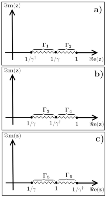
Figure 1 Branch cuts for the function F(z) for cases in which: a) CF > α > β, b) α > CF > β and c) α > β ¸ CF

which describes the discontinuities presented by the Rayleigh secular equation 28.

3.1.Case (a): CF>α>β

For this case the arcs over which the discontinuities spans (see Fig. 1a)) are

Γ1(t)=t,t1/γt1/γΓ2(t)=t,t1/γ<t1

The respective discontinuity quotient along each arc is described as

G1(t)=F+(t)F-(t)|Γ1=1+iH1(t)1-iH1(t),G2(t)=F+(t)F-(t)|Γ2=1-iH2(t)1+iH2(t) (11)

with the auxiliary functions

H1(t)=γ\dagρFρ1-γtγ\dagt-1γ(2t-1)2+4t1-t1-γt,H2(t)=4t1-tγt-1γ(2t-1)2+γ\dagρFργt-1γ\dagt-1. (12)

For the range of velocities under consideration, note that

limt1/γG1(t)Γ1=limt1/γG2(t)Γ2=1

guarantees the continuous continuation of these functions. The limit in which the fluid vanishes (ρF0) must satisfy

limρF0H1(t)|Γ1=0,limρF0H2(t)|Γ2=1-iHR(t)1+iHR(t)|ΓR. (13)

Where ΓR is described by Eq. (10) and

HR(t)=4t1-tγt-1γ(2t-1)2 (14)

is the auxiliary function for the free surface limit 28. Otherwise, the corresponding auxiliary functions are described by Eq. (12).

Moreover, it is prohibitive that γ=γ, since in vacuum the mechanical waves do not propagate. However, there is not physical restriction to consider a fluid medium with density ρF=ρ', where 0<ρ'1 for which exist an ϵ in the range 0<ϵ1 such that CF=α-ϵ. Then, at this limit we will have

limCFα-ϵH1(t)|Γ10,limCFα-ϵH2(t)|Γ2HR(t). (15)

Thus, while a fluid under which the solid-fluid interface may be defined, the contribution to the fluid discontinuities will be distinct to the free-surface limit.

3.2.Case (b): α>CF>β

For a fluid under this range of velocities, the discontinuities (see Fig. 1b)) are described by

G3(t)=F+(t)F-(t)|Γ3=1+iH3(t)1-iH3(t),G4(t)=F+(t)F-(t)|Γ4=1-iH4(t)1+iH4(t) (16)

with the auxiliary functions

H3(t)=γ(2t-1)24t1-tγt-1+γρFργt-1γt-1,H4(t)=4t1-tγt-1γ(2t-1)2+γρFργt-11-γt, (17)

which are defined along the arcs

Γ3(t)=t,  t  1/γ<t1/γ,Γ4(t)=t,  t  1/γt1. (18)

Here the continuous continuation and unicity of solutions is granted by

limt1/γG2(t)Γ3=limt1/γG3(t)Γ4=1,

while for the limit with ρF0 satisfies

limρF0H3(t)Γ3=0,  limρF0H4(t)Γ4=1-iHR(t)1+iHR(t) (19)

as in the previous case. Particularly for this case, note that the Rayleigh branch cut ΓR moves from partially screened to unscreened as the presence of a fluid vanishes (see Fig. 2a) and b)). Here HR(t) is described by Eq. (14). As in a previous case, it could be considered a fluid medium with density ρF=ρρ' in the range 0<ρ1 such that CF=α+ϵ, with 0<ϵ1. At this limit we will have

limCFα+ϵH3(t)|Γ1limCFα-ϵH1(t)|Γ10,andlimCFα+ϵH4(t)|Γ2limCFα-ϵH2(t)|Γ2HR(t). (20)

Thus the connection of discontinuities on both cases (a) and (b) is granted trough the free-surface limit.

Contrarily to the unscreened Rayleigh branch cut limit, the full-screening of ΓR occurs when γ1 (see Fig. 2c)) where

limγ1H4(t)Γ4=0,

and

limγ1H3(t)Γ3=γ(2t-1)24t1-tγt-1+ρFργt-11-t. (21)

then, the extreme values of 𝐺 3 (𝑡), particularly corresponds to well-defined values

limγ1G3t=1γ=-1,limγ1G3t=1=1.

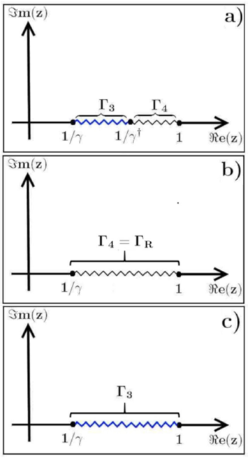
Figure 2 Branch cuts for the function F(z) in the case that α > C F > β for: a) the general case, b) p F → 0 and c) 1= y → 1. The branch cut colored in blue represents the fluid discontinuities’ contribution to the three different cases. The cases in which Γ R is totally unscreened and totally screened correspond to Figures b) and c) respectively. 

3.3.Case (c):α>βCF

Within this range of velocities, the discontinuities (see Fig. 1c)) are described by

G5(t)=F+(t)F-(t)Γ5=1+iH5(t)1-iH5(t),

G6(t)=F+(t)F-(t)Γ6=1+iH6(t)1-iH6(t) (22)

along the branch cuts

Γ5(t)=t,  t  1/γ<t1,Γ6(t)=t,  t  1<t1/γ. (23)

with the auxiliary functions

H5(t)=γ(2t-1)24t1-tγt-1+γρFργt-11-γt,H6(t)=γ(2t-1)2-4tt-1γt-1γρFργt-11-γt. (24)

It should be noted that the lowest value which 1/γ could take in this speed range is 1, which implies that not only the Rayleigh branch cut ΓR is always screened for this case, but are also extended beyond Re(z)>1 (See Fig. 1c)). Which is evident if it is observed that

limγ1G5(t)Γ5=limγ1G3(t)Γ3,limγ1G6(t)Γ6=0.

Which establishes the continuous continuation between G3 and G5. On the other hand, for the limit in which ρF0 we have

limρF0G5(t)Γ5=HR(t)+iHR(t)-i,limρF0G6(t)Γ6=-1. (25)

Here HR(t) is the auxiliary function defined by Eq. (14). Within this range, the discontinuities quotients are different to those obtained with the same limit in Eqs. (13) and (19). Similar expressions are obtained when γ0 is reached, however, their behavior along the arc Γ6 is not required to be similar; this is because, in general, we do not have a physical argument to establish a linear relation between p and CF.

4.The Scholte solution

Since we have guaranteed the continuous continuation of the Scholte discontinuities for the entire range of fluid velocities, we are in a position to determine the polynomial containing the zeros of Eq. (7). According to the construction 5 for the canonical solution of the Riemann problem, the polynomial with only zeros of the Scholte characteristic Eq. (7) is

Rz=2γ-1zγγz-2γ2+γ-124γγ-1+12γ+ρFγ1-δγ2ργ-1-Ia,b,c (26)

which was obtained through the Bourniston method . This method involves the expansion of Eq. (A.3) in terms of Laurent series. It should be noted that unlike previous works 19,27,29, the parametrization in terms of slowness conduces directly to a simple polynomial (26), and additional considerations are not necessary to solve it. In fact, directly from this polynomial is possible to have one and only one physical solution for the Scholte slowness, that is

zSc=βCSc2=2γ2+γ-124γ(γ-1)+12γ+ρFγ1-δγ2ργ-1-Ia,b,c (27)

Here δ is a correction parameter introduced to enhance the numerical accuracy of the Scholte root, which is a consequence of the truncation process during the Laurent series expansion (Eq. (7)). The Ia, Ib Ic terms represent the contribution of the discontinuities for the different speed ranges and are expressed in terms of Eqs. (12), (17) and (24) as

Ia=1πΓ1arctanH1tdt-Γ2arctanH2tdt, (28a)

Ib=1πΓ3arctanH3tdt-Γ4arctanH4tdt, (28b)

Ic=1πΓ5arctanH5tdt+Γ6arctanH6tdt. (28c)

4.1.The free surface limit

Contributions associated exclusively with the ΓR branch cut, occur only at the point at which the continuous continuation of the speed range between cases (a) and (b) occurs; i.e., the pole contribution. Thus, the free surface limit in terms of Eqs. (27), (28) and (28b) corresponds to

limρF0zSc=zR=2γ2+γ-124γ(γ-1)+1π1/γ1arctanHR(t)dt  (29)

Figure 3 Sholte (z Sc ) versus Rayleigh (z R ) slowness as function of the Poisson’s ratio. 

or explicitly to

zR=(βCR)2=2γ2+(γ-1)24γ(γ-1)+1π1/γ1arctan(4t1-tγt-1γ(2t-1)2)dt, (30)

which, according to 28, describes the exact slowness of the Rayleigh’s wave propagation. Note that the δ term is not included in this expression.

4.2.Numerical Results

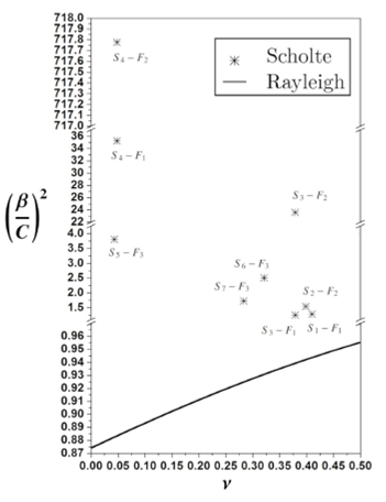
To numerically test the expression in Eq. (27) for different solid-fluid interfaces, we have used the parameters in Table I to illustrate the numerical derivation of the root in each of the three different fluid speed ranges. Wolfram Mathematica software was used to implement this expression numerically. The root calculated from Eq. (27) was compared with that obtained from Eq. (5) utilizing a root finder routine (provided by the software). It should be noted that not in all cases, the root finder routine was able to obtain the correct value, even when the provided value was close to the zero.

Table I Input parameters for the different solid (S i ) and fluid (F i ) materials under consideration. 

Material Label Density [Kg/m3] Compressional Speed [m/s] Shear Speed [m/s]
7-A teflon a S1 2157.7 1307 503
Lucite b S2 1180 2680 1100
Silver b S3 10400 3650 1610
Berylium b S4 1870 12890 8880
Ice-1 c S5 344 440 304
Ice-2 d S6 442 1472 755
Ice-3 e S7 637 2709 1489
Water (Distilled) b F1 998 1496 -
Air (dry) b F2 1.293 331.45 -
Sea Water f F3 1028.15 1442.45 -

aReference 35. bReference 36. cValues taken at sea level 37. dValues taken at 5 mts depth 37. eValues taken at 20 mts depth 37. f Density computed at sea level, 0oC, 30 PSU salinity and 1 Atm.38. Compressional speed taken from Ref.39.

Table II (for distinct solid-fluid interfaces) shows the corrected (δ0) and uncorrected (δ=0) zero values obtained. The precision of the corrected root (zSc(δ0)) in terms of the exact root (zSC*) was computed using,

Δ=F(zSC*)-F(zSc(δ0)).

Table II Values for the associated Poisson’s ratio º for each solid-fluid interface (Si ¡Fj ), corrected and uncorrected roots, the correction parameter ± and the precision of the corrected root ¢ associated to this parameter. 

Interface ν z Sc (Uncorrected) z Sc (Corrected) δ
S1 − F1 0.4103 1.33931 1.28279 0.54107 4.19 × 10⁻⁶
S2 − F2 0.3987 1.63185 1.54761 0.40354 2.78 × 10⁻⁶
S3 − F1 0.3792 1.34904 1.25176 3.702 6.6 × 10⁻⁶
S3 − F2 0.3792 23.69205 23.59477 2857.6 2.2 × 10⁻⁷
S4 − F1 0.04836 35.47909 35.24175 0.6781 6.3 × 10⁻⁶
S4 − F2 0.04836 718.29634 717.77757 1144.4 1.2 × 10⁻⁵
S5 − F3 0.0433 3.8311 3.8089 0.0112 3.18 × 10⁻⁶
S6 − F3 0.3215 2.6407 2.5092 0.1624 5.27 × 10⁻⁶
S7 − F3 0.2835 1.8804 1.7293 0.5555 2.36 × 10⁻⁶

The results are summarized in Table II. A direct comparison of these values shows that the uncorrected root presents a relative error ϵ with respect to the corrected one between 1%ϵ<7%. Thus, even for δ = 0 the predicted root presents a reasonable value. Finally, in Fig. 3, both zSc(δ0) and zR (computed from Eq. (30)) are plotted together to compare how the Scholte slowness increases for a particular interface (and v) in comparison with the Rayleigh slowness.

5.Conclusions

In terms of Cauchy integrals, we have obtained a robust analytic formula to predict the existence of a unique physical solution for the Scholte slowness in all range of possible elastic and isotropic media.The appropriated analysis of the discontinuities associated to the Scholte secular equation allows us to identify the free-surface limit as a pole contribution.

Unlike previous results 29, due to the secular Scholte equation’s fractional-order, our results show that the truncation process involved in obtaining the rational polynomial does not allow getting an exact solution. However, our numerical results show that this solution presents a reasonable approximation to the exact value. Additionally, since slowness is the inverse of speed, the results show that a Scholte wave’s propagation speed is less than or equal to that of a Rayleigh wave.

References

1. C. B. Park, R. D. Miller, and J. Xia, Multichannel analysis of surface waves, Geophysics 64 (1999) 800, https://doi.org/10.1190/1.1444590. [ Links ]

2. J. Xia, R. D. Miller, and C. B. Park, Estimation of nearsurface shearwave velocity by inversion of Rayleigh waves, Geophysics 64 (1999) 691, https://doi.org/10.1190/1.1444578. [ Links ]

3. D. Jongmans, and D. Demanet, The importance of surface waves in vibration study and the use of Rayleigh waves for estimating the dynamic characteristics of soils, J. Eng. Geol. 34 (1993) 105, https://doi.org/10.1016/0013-7952(93)90046-F. [ Links ]

4. G. Athanasopoulos, P. Pelekis, and G. Anagnostopoulos, Effect of soil stiffness in the attenuation of Rayleigh-wave motions from field measurements, Soil Dyn. Earthq. Eng. 19 (2000) 277, https://doi.org/10.1016/S0267-7261(00)00009-9. [ Links ]

5. C. G. Lai, G. J. Rix, S. Foti, and V. Roma, Simultaneous measurement and inversion of surface wave dispersion and attenuation curves, Soil Dyn. Earthq. Eng. 22 (2002) 923, https://doi.org/10.1016/S0267-7261(02)00116-1. [ Links ]

6. A. Hanyga, Seismic Wave Propagation in the Earth (Elsevier, New York, 1985), https://doi.org/10.1016/C2009-0-09602-0. [ Links ]

7. K. Aki, Keiiti, and Paul G. Richards, Quantitative Seismology, 2nd ed. (University Science Books, New Jersey, 2002), https://www.ldeo.columbia.edu/~richards/Aki_Richards.html. [ Links ]

8. E. Flores-Mendez et al., Interface Waves in Elastic Models Using a Boundary Element Method, J. Appl. Math 2012 (2012) 313207, https://doi.org/10.1155/2012/313207. [ Links ]

9. F. Luppé et al., Plane evanescent waves and interface waves, in Acoustic Interactions with Submerged Elastic Structures, edited by A. Guran, A. De Hoop, D. Guicking, and F. Mainardi (World Scientific, Singapore, 2001), pp. 118-148, https://doi.org/10.1142/9789812810755_0005. [ Links ]

10. A. Fahr, S. Johar, M. K. Murthy and W. R. Sturrock, Surface acoustic wave studies of surface cracks in ceramics, Review of Progress in Quantitative Nondestructive Evaluation, edited by D. O. Thompson and D. E. Chimenti (Springer, Boston, 1984), https://doi.org/10.1007/978-1-4684-1194-2. [ Links ]

11. M. J. Brophy, and A. V. Granato, Surface acoustic wave studies of defects in electron irradiated GaAs, J. Phys. Colloques 46 (1985) 541, https://doi.org/10.1051/jphyscol:198510120. [ Links ]

12. D. P. Morgan, A history of surface acoustic wave devices, Int. J. High Speed Electron. Syst. 10 (2000) 553, https://doi.org/10.1142/S0129156400000593. [ Links ]

13. J. Kondoh, Fundamentals and Applications of Surface Acoustic Wave Sensors, IEICE ESS Fundamentals Review 6 (2012) 166, https://doi.org/10.1587/essfr.6.166. [ Links ]

14. B. Liu et al., Surface acoustic wave devices for sensor applications, J. Semicond. 37 (2016) 021001, https://doi.org/10.1088/1674-4926/37/2/021001. [ Links ]

15. J. McLean and F. L. Degertekin, Directional scholte wave generation and detection using interdigital capacitive micromachined ultrasonic transducers, IEEE Trans Ultrason Ferroelect Freq Control 51 (2004) 756, https://doi.org/10.1109/TUFFC.2004.1304274. [ Links ]

16. M. Seidl, M. Gehring, U. Krumbein and G. Schrag, Simulation-based design of a micro fluidic transportation system for mobile applications based on ultrasonic actuation, 2018 19th International Conference on Thermal, Mechanical and Multi-Physics Simulation and Experiments in Microelectronics and Microsystems Toulouse, 2018, edited by IEEE (IEEE, Tolouse, 2018), https://doi.org/10.1109/EuroSimE.2018.8369873. [ Links ]

17. J. G. Scholte. On the stoneley wave equation. Proceedings of the Koninklijke Nederlandse Akademie van Wetenschappen 45 (1942) 159. [ Links ]

18. J. W. S. Rayleigh, On waves propagated along the plane surface of an elastic solid, Proc. London Math. Soc. 17 (1885) 4, https://doi.org/10.1112/plms/s1-17.1.4. [ Links ]

19. L. Knopoff, On rayleigh wave velocity, Bull. Seismol. Soc. Am. 42 (1952) 307, https://pubs.geoscienceworld.org/bssa/article-pdf/42/4/307/2691698/BSSA0420040307.pdf. [ Links ]

20. M. Romeo, Rayleigh waves on a viscoelastic solid half-space, J. Acoust. Soc. Am. 110 (2001) 59, https://doi.org/10.1121/1.1378347. [ Links ]

21. M. Hayes, and R. S. Rivlin, A note on the secular equation for Rayleigh Waves, Z. Angew. Math. Phys. 13 (1962) 80, https://doi.org/10.1007/BF01600759. [ Links ]

22. M. Rahman, and J. R. Barber, Exact expressions for the roots of the secular equation for Rayleigh waves, J. Appl. Mech. 62 (1995) 250, https://doi.org/10.1115/1.2895917. [ Links ]

23. X. F. Liu and Y. H. Fan, A New Formula for the Rayleigh Wave Velocity, Adv. Mater. Res. 452 (2012) 233, https://doi.org/10.4028/www.scientific.net/AMR.452-453.233. [ Links ]

24. P. G. Malischewsky, Comment to “A new formula for the velocity of Rayleigh waves” by D. Nkemzi [Wave Motion 26 (1997) 199-205], Wave Motion 31 (2000) 93, https://doi.org/10.1016/S0165-2125(99)00025-6. [ Links ]

25. X. -F. Liu, and Y.-h. Fan, A New Formula for the Rayleigh Wave Velocity, Adv. Mat. Res. 452 (2012) 233, https://doi.org/10.1016/S0165-2125(97)00004-8. [ Links ]

26. P. G. Malischewsky, Comment to “A new formula for the velocity of Rayleigh" waves by D. Nkemzi [Wave Motion 26 (1997) 199-205], Wave Motion 31 (2000) 93, https://doi.org/10.1016/S0165-2125(99)00025-6. [ Links ]

27. G. Caviglia, and A. Morro, Inhomogeneous waves in solids and fluids, 1st ed. (World Scientific, Singapore , 1992). [ Links ]

28. D. Nkemzi, A new formula for the velocity of rayleigh waves, Wave Motion 26 (1997) 199, https://doi.org/10.1016/S0165-2125(97)00004-8. [ Links ]

29. J. Antúnez-García, Master’s thesis, CICESE, Ensenada, Baja California, México (2003), http://cicese.repositorioinstitucional.mx/jspui/handle/1007/1589. [ Links ]

30. P. C. Vinh, Scholte-wave velocity formulae, Wave Motion 50 (2013) 180, https://doi.org/10.1016/j.wavemoti.2012.08.006. [ Links ]

31. R. Stoneley, Elastic waves at the surface of separation of two solids, Proc. Roy. Soc. London 106 (1924) 416, https://doi.org/10.1098/rspa.1924.0079. [ Links ]

32. J. G. Scholte, The range of existence of Rayleigh and Stoneley Waves, Geophys. Suppl. Mon. Nor. R. Astron. Soc. 5 (1947) 120, https://doi.org/10.1111/j.1365-246X.1947.tb00347.x. [ Links ]

33. I. A. Viktorov, Rayleigh and Lamb Waves, 1st ed. (Springer, New York, 1967). [ Links ]

34. E. Strick, and A. S. Ginzbarg, Stoneley-wave velocities for a fluid-solid interface, Bull. Seismol. Soc. Am. 46 (1956) 281. [ Links ]

35. E. E. Burniston, and C. E. Siewert, The use of Riemann problems in solving a class of transcendental equations, Math. Proc. Cambridge Philos. Soc. 73 (1973) 111, https://doi.org/10.1017/S0305004100047526. [ Links ]

36. P. J. Rae, and D. M. Dattelbaum, The properties of poly(tetrafluoroethylene) (PTFE) in compression, Polymer 45 (2004) 7615, https://doi.org/10.1016/j.polymer.2004.08.064. [ Links ]

37. D. R. Lide, CRC Handbook of Chemistry & Physics 89th ed. (Taylor and Francis, London, 2008). [ Links ]

38. C. R. Bently, The Ross Ice Shelf Geophysical and Glaciological Survey (RIGGS): Introduction and summary of measurements performed, in The Ross Ice Shelf: Glaciology and Geophysics, edited by C. R. Bentley and D. E. Hayes (American Geophysical Union, Washington D. C., 1990). [ Links ]

39. F. J. Millero, History of the Equation of State of Seawater, Oceanography 23 (2010) 18, https://doi.org/10.5670/oceanog.2010.21. [ Links ]

40. F. J. Millero, and T. Kubinski, Speed of sound in seawater as a function of temperature and salinity at one atmosphere, J. Acoust. Soc. Am. 57 (1975) 312, https://doi.org/10.1121/1.380462. [ Links ]

41. P. Henrici, Computational Complex Analysis, Vol. II, Willey, New York, (1984). [ Links ]

42. E. E. Burniston, and C. E. Siewert, Exact analytical solutions of the transcendental equation αsinζ = ζ, SIAM J. Appl. Math 24 (1973) 460, https://www.jstor.org/stable/2099816. [ Links ]

Appendix

A. The method based on Cauchy integrals

Let us consider a multivalued (or discontinuous) function F(z) with a pole of finite order at infinity. If we define a Riemann function for this sheet, it would be analytical (except at infinity) with its discontinuities isolated and their branch cuts. Thus, Privalov’s theory allows us to rewrite this function in terms of their canonical representation, as

F(z)=R(z)eg(z), (A.1)

where

g(z)=12πiΓlnG(t)t-zdt. (A.2)

Here R is a rational function that contains the zeros and poles of F, G is the quotient of the lateral limits F(t)+ and F(t)- along the arc Γ (which describes the branch cuts of F), and it is defined as

G(t)=F+(t)F-(t).

Since eg(z)0 in all the complex domain, it is directly observed from Eq. (A.1) that R admits the representation

R(z)=F(z)e-g(z). (A.3)

If the discontinuities of F are isolated at infinity, we could ensure that R contains this function’s zeros. In other words, we may obtain a polynomial representation for the zeros of F in terms of a Laurent series expansion 34,41.

Received: August 04, 2020; Accepted: September 29, 2020

Creative Commons License This is an open-access article distributed under the terms of the Creative Commons Attribution License