SciELO - Scientific Electronic Library Online

 
vol.66 número6Influence of pairing and deformation on charge exchange transitionsInformation entropies for H2 and ScF diatomic molecules with Deng- Fan-Eckart potential índice de autoresíndice de materiabúsqueda de artículos
Home Pagelista alfabética de revistas  

Servicios Personalizados

Revista

Articulo

Indicadores

Links relacionados

  • No hay artículos similaresSimilares en SciELO

Compartir


Revista mexicana de física

versión impresa ISSN 0035-001X

Rev. mex. fis. vol.66 no.6 México nov./dic. 2020  Epub 31-Ene-2022

https://doi.org/10.31349/revmexfis.66.730 

Research

Atomic and Molecular Physics

Arbitrary l -solutions of the Schrödinger equation interacting with Hulthén-Hellmann potential model

E. S. William1 

E. P. Inyang1 

E. A. Thompson1 

1Theoretical Physics Group, Department of Physics, University of Calabar, PMB 1115, Calabar, Nigeria. e-mail: williameddyphysics@gmail.com


Abstract

In this study, we obtain bound state solutions of the radial Schrödinger equation by the superposition of Hulthén and Hellmann potentials within the framework of Nikiforov-Uvarov (NU) method for arbitrary-state, with the Greene-Aldrich approximation for the centrifugal term. We also obtain the corresponding normalized wave functions expressed in terms of Jacobi polynomials for a particle exposed to this potential field. Explicitly, we have computed the numerical energy eigenvalues of different quantum states. Besides, we consider six exceptional cases of the potential and obtained their energy eigenvalues. Our results are in excellent agreement with the results in the literature. The behavior of the energy for the ground state and several excited states is illustrated graphically.

Keywords: Schrödinger equation; Nikiforov-Uvarov method; eigenvalues; eigenfunction; Hulthén-Hellmann potential

PACS: 03.65.w; 03.65.Fd; 03.65.Ge

1.Introduction

In the earlier study of quantum mechanics, the Schrödinger equation was introduced as a second-order differential equation capable of describing the properties of a non-relativistic Quantum system1-2. Studies have revealed that exact solutions of the Schrödinger equation are available only for a limited set of physical and chemical quantum mechanical systems 3-4. Hence, with an approximation to the centrifugal term, interest is geared towards arbitrary ℓ-solutions of the radial Schrödinger equation. Arbitrary l -solutions play a dominant role in non-relativistic quantum mechanics since the wave function and associated eigenvalues contain all the necessary information for a full description of a quantum system 5-8. With the experimental verification of the Schrödinger equation, researchers have devoted much interest in solving the radial Schrödinger equation to obtain bound state solutions with various methods for some potential models 9-25.

The Hulthén potential 26 is one of the essential short-range potentials in physics. Its application to diverse areas of physics, including nuclear and particle physics, atomic physics, condensed matter physics, and chemical physics, has been of great interest in recent times 27-29. The study of this potential is essential in investigating the interaction existing between two particles 30. The superposition of Yukawa and Coulomb potential, otherwise known as Hellmann potential 31, has been extensively used by many authors to obtain the energy of the bound state in atomic, nuclear, and particle physics 32-41. The Hellmann potential is useful in the study of transitions of alkali metal molecules in condensed matter physics.

Recently, a lot of interest has been directed towards combining two or more potentials in relativistic and non-relativistic regimes 35. The essence of combining two or more physical potential models is to have a broader range of applications 36. Hence, in the present study, we attempt to study the radial Schrödinger equation with a newly proposed potential, obtained from a combination of Hulthén and Hellmann’s potential (HHP). The potential is of the form:

V(r)=-Λ1e-αr1-e-αr-Λ2r+Λ3e-αrr, (1)

where r represents the inter-nuclear distance; Λ1, Λ2, and Λ3, and are the strengths of Hulthén, Coulomb, and Yukawa potentials, respectively, and a is the screening parameter. The shape of this potential as a function of r for varying screening parameters is presented in Fig. 1. It is obvious that the developed potential model works perfectly for both small and medium inter-nuclear distance.

Figure 1 The shape of Hulth´en-Hellmann’s potential as a function of r for different screening parameters. We choose Λ1 = 0:015, Λ2 = 2 and Λ3 = -2. 

2.Review of Nikiforov-Uvarov method

In this section, we briefly introduce the NU method. The details can be found in the Nikiforov-Uvarov handbook 42. This method is useful to solve the second-order differential wave equation of the hypergeometric type:

ψ(s)+τ̃(s)σ(s)ψ'(s)+σ̃(s)σ2(s)ψ(s)=0, (2)

where σ(s) and σ̃(s) are polynomials at most second-degree and τ̃(s) is a first-degree polynomial. The particular solution of Eq. (2) can be obtained by decomposing the wave function ψ(s) as follows:

ψ(s)=ϕ(s)y(s), (3)

leading to a hypergeometric-type equation

σ(s)y(s)+τ(s)y'(s)+λy(s)=0. (4)

The first part of the wave functions ψ(s) is the solution of the differential equation,

σ(s)ϕ'(s)-π(s)ϕ(s)=0, (5)

where

τ(s)=τ̃(s)+2π(s), (6)

and λ in Eq. (4) is the parameter defined as

λ=λn=-nτ´s+nn-12σ´´ s=0, (n=0,1,2,) (7)

The τ(s) is a polynomial function of the parameter 𝑠 whose first derivative τ'(s) must be negative. This is the essential condition in choosing the proper solutions. That is:

dτ(s)ds<0. (8)

The second part of the wave functions in Eq. (3) is a hypergeometric-type function obtained by Rodrigues relation:

yn(s)=Bn(s)ρ(s)dndsn[σn(s)ρ(s)], (9)

where Bn(s) is a constant related to normalization, and the weight function p(s) can be found by 42

dds[σ(s)ρ(s)]=τ(s)ρ(s). (10)

We define the function π(s) and the parameter λ as

πs=σ´s-τ~(s)2

±σ´s-τ~(s)22-τ~s+kσs, (11)

and

λ=k+π'(s), (12)

where π(s) has to be a polynomial of degree at most one.

The discriminant under the square root sign in Eq. (10) must be set to zero and then has to be solved for k 42. Finally, by solving Eqs. (7) and (12), the energy eigenvalue equation can be obtained.

2.1.Arbitrary l-solution to the radial Schrödinger equation

To obtain the solution of the Schrödinger-like equation given in Eq. (2), we write the radial Schrödinger equation of the form 15,41,43

d2ψnl(r)dr2+2μ2×Enl-Vr-2ll+12μr2ψnlr=0, (13)

where we have defined μ as the reduced mass, Enl as the energy spectrum, as the reduced Planck’s constant, V(r) as the interacting potential, l(l+1)/r2 as the centrifugal term, n and l as the radial and orbital angular momentum quantum numbers, respectively. Whenl=0, Eq. (13) with HHP can be exactly solved, but for the case l0, Eq. (13) cannot be solved exactly with the proposed potential. So we introduce the Greene-Aldrich approximation scheme 4,15,41,44 to deal with the centrifugal barrier in solving the equation analytically. This approximation scheme is a good approximation to the centrifugal term which is valid for α1, and it becomes

1r2α2(1-e-αr)2. (14)

Inserting the potential in Eq. (1) and applying the approximation scheme in Eq. (14), one can obtain

d2ψnl(r)dr2+2μ2Enl+Λ1e-αr1-e-αr+Λ2α1-e-αr-Λ3αe-αr1-e-αr-22μll+1α21-e-αr2ψnlr=0 (15)

By using the change of variable from rs, our new coordinate becomes

s=e-αr. (16)

We substitute Eq. (16) into Eq. (15) and after some simplifications, we have:

d2ψ(s)ds2+1-ss(1-s)dψ(s)ds+1s(1-s)2×-ς+k1-k3s2+2ς+k1-k2-k3s-ς-k2+k-4ψs=0 (17)

where

-ς=2μEnlα22,    k1=2μΛ1α22,    k2=2μΛ2α2,    k3=2μΛ3α2,  k4=l(l+1) (18)

Comparing Eqs. (17) and (2), we obtain the relevant polynomials as:

*20cτ̃=1-s;σ(s)=s(1-s);σ'(s)=1-2s;σ(s)=-2;σ(s)=-(ς+Λ1-Λ3)s2+(2ς+Λ1-Λ2-Λ3)s-(ς-Λ2+k4) (19)

Inserting the polynomials given by Eq. (19) into Eq. (11) gives the polynomial:

π(s)=-s2±(ω1-K)s2+(K-ω2)s+ω3, (20)

where

ω1=(14+ς+k1-k3),ω2=(2ς+κ1-k2-k3),ω3=(ς-k2+k4)}. (21)

According to the NU method, the quadratic form under the square root sign of Eq. (20) must be solved by setting the discriminant of this quadratic equation equal to zero: Δ=b2-4ac=0. This discriminant gives a new quadratic equation, which can be solved for the constant k to get the two roots. Here, we take the negative root given as:

K=-(ω2+2ω3)-2ω3ω3+ω2+ω1. (22)

Since τ(s) given in Eq. (6) has a negative derivative in Eq. (8) for this value of π(s) 42, π(s) has the most suitable expression given as

π(s)=-s2-[(ω3+ω3+ω2+ω1)s-ω3], (23)

using Eq. (22). Therefore, we obtain τ(s) and τ'(s) as follows:

τs=1-2s-2w3 s-2×w3+w2+η1+2w3 (24)

τ´s=-21+w3+w3+w2+w1 (25)

where τ'(s) is the first derivative of τ(s). Using Eqs. (19), (23), (24) and (25), the following expressions for λ n and λ are as follows:

λn=n2+1+2w3+2w3+w2+w1n, n=0,1,2,, (26)

λ=-12-w3-w3+w2+w1-w2+2w3-2w3w3+w2+w1, (27)

where n is the number of nodes in the radial wavefunctions ψnl. When comparing Eqs. (26) and (27) with the help of Eq. (18), we obtain bound state energy eigenvalues of HHP as:

Enl=α22l(l+1)2μ-Λ2α-α228μ×n+l+12+2μΛ3α2-2μΛ2α2-2μΛ1α22+l(l+1)n+l+12 (28)

We can obtain the other part of the wave function ϕ(s) and weight function p(s) by inserting the values of σ(s), π(s) and τ(s) given in Eqs. (19), (23) and (34) respectively into Eqs. (5) and (10) as follows:

ϕ(s)=sω3(1-s)(1/2+ω3+ω2+ω1), (29)

ρ(s)=s2ω3(1-s)(2+ω3+ω2+ω1). (30)

Using Eq. (30), the Rodrigues relation in Eq. (9) is written as:

Yn=Bns-2w3(1-s)2w3+w2+w1dndsn×sn1-sns2w31-s-2w3+w2+w1 (31)

where Bn is the Jacobi polynomial; hence, the wave function in Eq. (3) becomes:

ψnls=Nnlsw31-s1/2+w3+w2+w1×Pn2w3+w2+w1 (32)

where N nl is the normalization constant. Using the normalization condition, we obtain the normalization constant as follows:

Nnl2α-111-δ22w31+δ2β×Pn2w3,2β-1δ2dY=1 (33)

where

*20cβ=1+4ω3+4ω2+4ω1,β-1=4ω3+4ω2+4ω1 (34)

Comparing Eq. (33) with the standard integral of the form of Eq. (37) of 41,

-111-p2x1+y2y(Pn2x,2y-1(p))2dp=2Γ(x+n+1)Γ(y+n+1)n!xΓ(x+y+n+1). (35)

Hence, we write the normalization constant as

Nnl=n!2ω3αΓ(2ω3+4ω3+4ω2+4ω1+n+2)2Γ(2ω3+n+1)Γ(4ω3+4ω2+4ω1+n+2)1/2. (36)

3.Discussion

In Table I, we have reported some numerical results of the energy (eV) levels of Hulthén-Hellmann potential for various values of the potential strength: Λ1=0.025, Λ2=2, Λ3=1; Λ1=0.050, Λ2 =2; Λ3= -1 and Λ1=0.15, Λ2 =2, V2=-2 , respectively, as a function of the screening parameter for =2μ=1. The results show that the energy decreases as the screening parameter, and the potential strength increase. We have plotted the graph of energy eigenvalues as a function of the potential strength, screening parameter, and the reduced mass in the ground and excited states. From Figs. 2a) and b) - Figs. 4a) and b) respectively, we plotted the ground and excited states energy eigenvalues of the different quantum states as a function of the Hulthen, Coulomb, and Yukawa potential strengths, respectively. We observed that there is a decrease in energy in both the ground and excited states as the potential strength, Λ1, Λ2, and Λ3, increases respectively. This is well distinguished, especially in excited states.

Table I Energy eigenvalues (eV) of the Hulthén-Hellmann potential with =2, μ = 1 

state α Λ1 = 0.025, Λ2 = 1, Λ3 = −1 Λ1 = 0.050, Λ2 = 2, Λ3 = −2 Λ1 = 0.015, Λ2 = 4, Λ3 = −4
1s 0.025 -2.237656250 -8975156250 -48.92515625
0.050 -1.550625000 -6.225625000 -30.17562500
0.075 -1.350017362 -5.420850695 -2492640624
0.10 1.255625000 -5.040000000 -22.49000000
0.15 -1.166736110 -4.675069442 -20.18062500
2s 0.025 -0.5506250000 -2.225625000 -12.17562500
0.050 -0.3806250000 -1.540000000 -7.49000000
0.075 -0.3334027780 -1.341736111 -4333402775
0.10 -0.3139062500 -1.250625000 -5.575625000
0.15 -0.3034027778 -1.171111110 -5.010000000
2p 0.025 -0.5314062500 -2.187656250 -12.08765625
0.050 -0.3475000000 -1.475625000 -7.350625000
0.075 -0.2854340280 -1.250017360 -5.988906248
0.10 -0.2501562500 -1.130625000 -5.330625000
0.15 -0.2052777777 -0.9917361105 -4.655625000
3s 0.025 -0.2389062500 -0.9764062500 -5.370850695
0.050 -0.1667361111 -0.67506494445 -3.291736110
0.075 -0.1513908180 -0.5925945218 -2.715434026
0.10 -0.1506250000 -0.5600000000 -2.454444445
0.15 -0.1685262345 -0.5472299380 -2.225625000
3p 0.025 -0.2300173611 -0.9591840278 -5.331406250
0.050 -0.1506250000 -0.645069445 -3.228402778
0.075 -0.1269463735 -0.5487056328 -2.627100694
0.10 -0.1167361111 -0.5011111110 -2.340000000
0.15 -0.1124151234 -0.4550077159 -2.055625000
3d 0.025 -0.2126562500 -0.9251562500 -5.252934028
0.050 -0.1200694444 -0.5867361110 -30103402778
0.075 -0.08180748460 -0.4646778548 -2.454184026
0.10 -0.05562500000 -0.3900000000 -2.117777778
0.15 -0.01519290124 -0.2855632714 -1.730625000
4s 0.025 -0.13062500000 -0.5400000000 -2.990000000
0.050 -0.09515625000 -0.3756250000 -1.825625000
0.075 -0.09506944448 -0.3377777778 -1.509999999
0.10 -0.1066015625 -0.3314062500 -1.375156250
0.15 -0.1508506944 -0.3584027777 -1.280625000
4p 0.025 -0.1253515625 -0.5300390625 -2.967539062
0.050 -0.08500000000 -0.3576562500 -1.788906250
0.075 -0.07885850696 -0.3106293402 -1.457851562
0.10 -0.08316406250 -0.2939062500 -1.306406250
0.15 -0.1094444445 -0.2966840277 -1.175156250

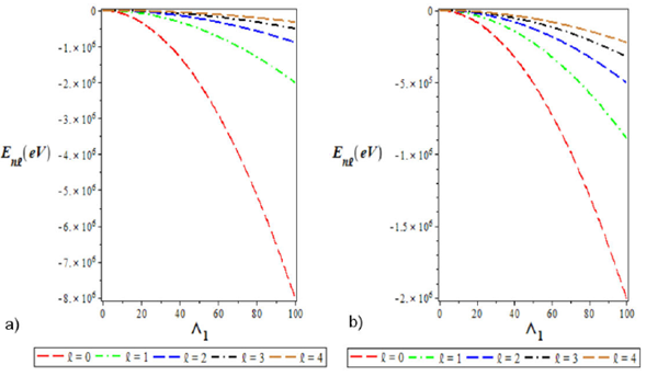
Figure 2 a). Variation of the ground state energy spectra for various l as a function of Λ1 . b). The plot of the first excited state energy spectra for different l as a function of Λ1. We choose Λ1 = 0:10, Λ2 = 4, Λ3 = -4, and a = 0:025 for the ground and excited states. 

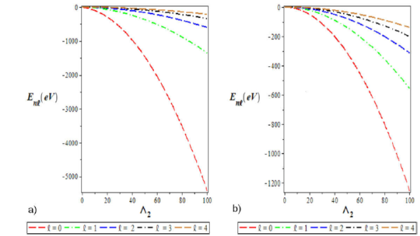
Figure 3 a) Variation of the ground state energy spectra for various l as a function of Λ2. b) A plot of the first excited state energy spectra for various l as a function of Λ2. We choose Λ1 = 0:10, Λ2 = 4, Λ3 = -4, and a = 0:025 for the ground and excited states. 

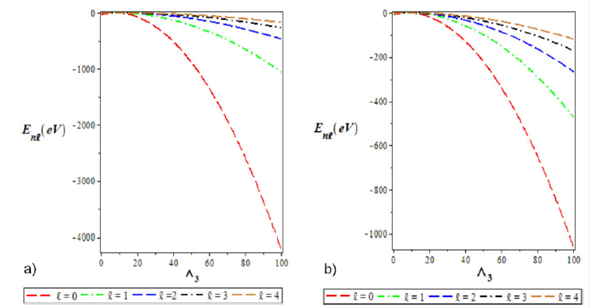
Figure 4 a) Variation of the ground state energy spectra for various l as a function of Λ3. b) The plot of the first excited state energy spectra for various l as a function of Λ3. We choose Λ1 = 0:10, Λ2 = 4, Λ3 = -4, and a = 0:025 for the ground and excited states. 

In Fig. 5a) and 5b), we graphically show the variation of energy eigenvalues of HHP as a function of the screening parameter. Here, the energy eigenvalue increases with a small screening parameter (α1, the limit of our screening parameter) and is invariant as the screening parameter becomes larger in the ground and excited states. In Fig. 6a) and 6b), there is a decrease in the ground and excited states energy eigenvalues for different quantum states as the reduced mass, μ increases.

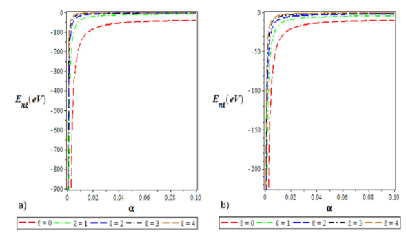
Figure 5 a) Variation of the ground state energy spectra for various l as a function of the screening parameter (a). b) A plot of the first excited state energy spectra for different l as a function of the screening parameter (a). We choose Λ1 = 0:10, Λ2 = 4, Λ3 = -4, and a = 0:025 for the ground and excited states. 

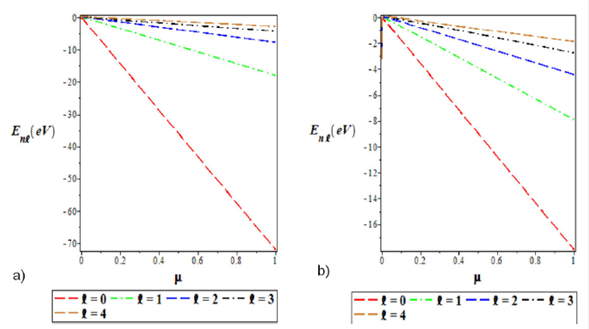
Figure 6 a) Variation of the ground state energy spectra for various l as a function of the screening parameter (μ). b) A plot of the first excited state energy spectra for different l as a function of the reduced mass (μ). We choose Λ1 = 0:10, Λ2 = 4, Λ3 = -4, and a = 0:025 for the ground and excited states. 

4.Special cases

4.1.Hellmann potential

If we set the parameter Λ1 = 0, the Hulthén-Hellmann potential in Eq. (1) reduces to Hellmann potential of the form

V(r)=-Λ2r+Λ3e-αrr, (37)

hence, its corresponding energy eigenvalue is of the form

Enl=α22l(l+1)2μ-Λ2α-α228μ×n+l+12+2μα2Λ3-Λ2+l(l+1)n+l+12 (38)

Equation (38) is in agreement with Eq. (39) of 15. In Table II and Table III, we present the numerical energy eigenvalues for Hellman potential for (Λ1 = 0, Λ2 = 2, Λ2 = 1) and (Λ1 = 0, Λ2 = 5, Λ3 = -1), respectively. The results showed good agreement with the earlier results of 19 with NU, AP, and SUSY methods of 45 and PT method of 46.

Table II Comparison of energy eigenvalues (eV) for a particular case of Hellmann potential as a function of the screening parameter α with = 2µ = 1 for Λ1 = 0, Λ2 = 2, and Λ3 = 1. 

State α Present method (SUSY) [45] (NU) [19] (AP) [19] (PT) [46]
1S 0.001 -0.2515002500 -0.251500 -0.251500 -0.250969 -0.250999
0.005 -0.2575062500 -0.257506 -0.257506 -0.254933 -0.254963
0.01 -0.2650250000 -0.265025 -0.265025 -0.259823 -0.289852
2S 0.001 -0.06400100000 -0.064001 -0.064001 -0.063243 -0.063494
0.005 -0.07002500000 -0.070025 -0.070025 -0.067106 -0.067353
0.01 -0.07760000000 -0.077600 -0.077600 -0.071689 -0.071928
2P 0.001 -0.06375025000 -0.063750 -0.064000 -0.063495 -0.063495
0.005 -0.06875625000 -0.068756 -0.070000 -0.067377 -0.067377
0.01 -0.07502500000 -0.075025 -0.077500 -0.072020 -0.072020
3S 0.001 -0.02928002778 -0.029280 -0.029280 -0.028283 -0.028764
0.005 -0.03533402778 -0.035334 -0.035334 -0.031993 -0.032457
0.01 -0.04300277778 -0.043003 -0.043003 -0.036142 -0.036557
3P 0.001 -0.02916802778 -0.029169 -0.029279 -0.028765 -0.028765
0.005 -0.03475625000 -0.034756 -0.035309 -0.032480 -0.032480
0.01 -0.04180277778 -0.041803 -0.042903 -0.036648 -0.036644
3d 0.001 -0.02894469445 -0.028945 -0.029388 -0.028767 -0.250833
0.005 -0.03361736111 -0.033617 -0.035817 -0.032526 -0.254151
0.01 -0.03946944445 -0.039469 -0.043825 -0.036813 -0.258269
4S 0.001 -0.01712900000 -0.017129 -0.029280 -0.016130 -0.016601
0.005 -0.02322500000 -0.023225 -0.035334 -0.019646 -0.020077
0.01 -0.03102500000 -0.031025 -0.043003 -0.023289 -0.023551
4p 0.001 -0.01706556250 -0.017066 -0.017128 -0.016602 -0.016602
0.005 -0.02288906250 -0.022889 -0.023200 -0.020100 -0.020098
0.01 -0.03030625000 -0.030306 -0.030925 -0.023711 -0.023641
4d 0.001 -0.01693906250 -0.016939 -0.017189 -0.016604 -0.016604
0.005 -0.02222656250 -0.022227 -0.023464 -0.020142 -0.020142
0.01 -0.02890625000 -0.028906 -0.031356 -0.023857 -0.023814
4f 0.001 -0.01675025000 -0.016750 -0.017311 -0.016607 -0.016607
0.005 -0.02125625000 -0.021257 -0.024027 -0.020206 -0.020206
0.01 -0.02690000000 -0.026900 -0.032356 -0.024072 -0.024056

TableIII Comparison of energy eigenvalues (eV) for a particular case of Hellmann potential as a function of the screening parameter α with = 2µ = 1 for Λ1 = 0, Λ2 = 2, and Λ3 = −1. 

State α Present method (NU) [19] (AP) [19] (PT) [46]
1S 0.001 -2.250500250 -2.250500 - 2.248981 - 2.24900
0.005 -2.252506250 -2.252506 - 2.244993 - 2.24501
0.01 -2.255025000 -2.255025 - 2.240030 - 2.24005
2S 0.001 -0.5630010000 - 0.563001 - 0.561502 - 0.561502
0.005 -0.5650250000 - 0.565025 - 0.557549 - 0.557550
0.01 -0.5676000000 - 0.567600 - 0.552697 - 0.552697
2P 0.001 -0.5622502500 - 0.563000 - 0.561502 - 0.561502
0.005 -0.5612562500 - 0.565000 - 0.557541 - 0.557541
0.01 -0.5600250000 - 0.567500 - 0.552664 -0.552664
3S 0.001 -0.2505022500 - 0.250502 - 0.249004 - 0.249004
0.005 -0.2525562500 - 0.252556 -0245110 - 0.245111
0.01 -0.2552250000 - 0.255225 -0.240435 - 0.240435
3p 0.001 -0.2501680278 -0.250501 - 0.249004 - 0.249004
0.005 -0.2508673611 -0.252531 -0.245102 -0.245103
0.01 -0.2518027778 -0.255125 -0.240404 -0:240404
3d 0.001 -0.2495002500 -0.250833 -0.249003 -0.249003
0.005 -0.2475062500 -0.254151 -0.245086 -0.245086
0.01 -0.2450250000 -0.258269 -0.240341 -0.240341
4S 0.001 -0.1411290000 -0.141129 -0.139633 -0.139633
0.005 -0.1432250000 -0.143225 -0.135819 -0.135819
0.01 -0.1460250000 -0.146025 -0.131380 -0.131381
4p 0.001 -0.1409405625 -0.141128 -0.139632 0.139633
0.005 -0.1422640625 -0.143200 -0.135811 0.135811
0.01 -0.1440562500 -0.145925 -0.131350 -0.131351
4d 0.001 -0.1405640625 -0.141314 -0.139632 -0.139632
0.005 -0.1403515625 -0.144089 -0.135795 -0.135796
0.01 -0.1401562500 -0.147606 -0.131290 -0.131290
4f 0.001 -0.1400002500 -0.141686 -0.139631 -0.139631
0.005 -0.1375062500 -0.145902 -0.135772 -0.135772
0.01 -0.1344000000 -0.151106 -0.131200 -0.131200

4.2.Hulthén potential

If we set Λ2 = Λ3 = 0, the Hulthén-Hellmann potential in Eq. (1) reduces to Hulthén potential

V(r)=-Λ1e-αr1-e-αr, (39)

where Λ1=Ze2α is the strength of Hulthén potential, Z is the atomic number, 𝑒 is the electronic charge, and a is the screening parameter 5. Making the same substitution into Eq. (27), the energy eigenvalues of Hulthén potential becomes:

Enl=α22l(l+1)2μ-α228μ×n+l+12+2μΛ1α22+l(l+1)(n+l+1)2 (40)

Equation (40) is in agreement with Eq. (41) of 47, Eq. (32) of 48; Eq. (24) of 49; Eq. (28) of 32; Eq. (37) of 50 and Eq. (20) of 16. Table IV is the numerical energy eigenvalues of Hulthén potential for 2p, 3p, 3d, and 4p with =μ=e=1 and for Z =1. We compare the results with those obtained with AIM 43, EQR 51, and SUSY 52. Our results obtained with the Greene-Aldrich approximation scheme for small screening parameters using the NU method are in excellent agreement with those obtained by other methods.

Table IV Comparison of energy eigenvalues (eV) of the Hulthén potential as a function of the screening Parameters α for 2p, 3p, 3d, and 4p states and for Z = 1 in atomic units ( = µ = e = 1). 

State α Present (NU) AIM [43] EQR [51] SUSY [52]
2p 0.025 -0.1128125000 -0.1128125 -0.1128125 -0.1127605
0.050 -0.1012500000 -0.1012500 -0.1012500 -0.1010425
0.075 -0.09031249994 -0.0903125 -0.0903125 -0.0898478
0.10 -0.08000000000 -0.0800000 -0.0800000 -0.0791794
0.15 -0.06124999998 -0.0612500 -0.0612500 -0.0594415
3p 0.025 -0.04070312500 -0.0437590 -0.0437590 -0.0437068
0.050 -0.03336810000 -0.0333681 -0.0333681 -0.0331632
0.075 -0.02438370000 -0.0243837 -0.0243837 -0.0239331
0.10 -0.01680560000 -0.0168056 -0.0168056 -0.0160326
0.15 -0.00586810000 -0.0058681 -0.0058681 -0.0043599
3d 0.025 -0.04360440000 -0.0437587 -0.0437587 -0.0436030
0.050 -0.03275080000 -0.0333681 -0.0333681 -0.0327532
0.075 -0.02299480000 -0.0243837 -0.0243837 -0.0230306
0.10 -0.01433640000 -0.0162600 -0.0162600 -0.0144832
0.15 -0.00031240000 -0.0058681 -0.0058681 -0.0132820
4p 0.025 -0.01994860000 -0.0200000 -0.0200000 -0.0199480
0.050 -0.01104420000 -0.0112500 -0.0112500 -0.0110430
0.075 -0.00453700000 -0.0050000 -0.0050000 -0.0045385
0.10 -0.00042690000 -0.0012500 -0.0012500 -0.0004434

4.3.Hulthén-Yukawa potential

If we set Λ2 = 0 the Hulthén-Hellmann potential in Eq. (1) reduces to Hulthén-Yukawa potential

V(r)=-Λ1e-αr1-e-αr+Λ3e-αrr. (41)

Similarly, Eq. (27) reduces to the energy equation for the Hulthén-Yukawa potential

Enl=α22l(l+1)2μ-α228μ×n+l+12+2μΛ3α22-2μΛ1α22l(l+1)(n+l+1)2 (42)

Equation (42) is in agreement with Eq. (24) of 43.

4.4.Hulthén-Coulomb potential

If we set Λ3 = 0, the Hulthén-Hellmann potential in Eq. (1) reduces to Hulthén-Coulomb potential

V(r)=-Λ1e-αr1-e-αr-Λ2r. (43)

Equation (27) reduces to energy eigenvalues of Hulthén-Coulomb potential.

Enl=α22l(l+1)2μ-Λ2α-α228μ×n+l+12+2μΛ2α22-2μΛ1α22l(l+1)(n+l+1)2 (44)

4.5.Yukawa Potential

When the potential strength of Hulthén and Coulomb potentials are equal to zero, i.e., Λ1 = Λ2 = 0 the Hulthén-Hellmann potential in Eq. (1) reduces to the Yukawa potential

V(r)=-Λ3e-αrr, (45)

with the corresponding energy eigenvalues obtained from Eq. (27) as

Enl=α22l(l+1)2μ-α228μ×n+l+12+2μΛ3α22+l(l+1)(n+l+1)2 (46)

Equation (46) is in agreement with Eq. (34) of 16.

4.6.Coulomb potential

If we set Λ1 = Λ2 = a =0, the Hulthén-Hellmann potential in Eq. (1) reduces to the familiar Coulomb potential

V(r)=-Λ2r, (47)

and we write the energy eigenvalues as

Enp=Z2e4μ22np2, (48)

where the principal quantum number, n p = (n + l + 1), and Λ2=Ze2 is the nuclear charge. Equation (48) agrees with Eq. (39) of 16; and Eq. (16) of 51.

5.Conclusion

In this work, we have studied the bound state solutions of the Schrödinger equation for any arbitrary l-state by the superposition of Hulthén and Hellmann potentials using the Nikiforov-Uvarov method. After making appropriate approximation to the centrifugal barrier, we obtained the energy eigenvalues and the corresponding normalized wave functions. We also considered six special cases of the potential and obtained their energy eigenvalues. Our results are in excellent agreement with the results in the literature. Also, we have presented plots of energy eigenvalues for various values of the potential parameters in the ground and excited states.

References

1. W. Greiner, Quantum Mechanics, An Introduction 4th Ed. (Springer-Verlag Berlin, New York, 2001). https://doi.org/10.1007/978-3-642-56826-8. [ Links ]

2. C. Cari, A. Suparmi, and H. Azizah, The approximate solution of Schrödinger equation with minimal length presence for Yukawa potential, AIP Conf. Proc. 2014 (2018) 020093, https://doi.org/10.1063/1.5054497 [ Links ]

3. C. P. Onyenegecha, C. A. Onate, O. K. Echendu, A. A. Ibe, and H. Hassanabadi, Solutions of Schrödinger equation for the modified Mobius square plus Kratzer potential. Eur. Phys. J. Plus 135 (2020) 289, doi:10.1140/epjp/s13360-020-00304-z [ Links ]

4. R. H. Parmar, K. R. Purohit, and A. K. Rai, Approximaate analytical solution of the extended Hulthen-Yukawa with inverse square and Coulombic term plus ring shape potential, AIP Conf. Proc. 2220 (2020) 140071. https//doi.org/10.1063/5.0001432 [ Links ]

5. H. I. Ahmadov, M. V. Qocayeva, and N. Sh. Huseynova, The bound state solutions of the D-dimensional Schrödinger equation for the Hulthén potential within SUSY quantum mechanics. Int. J. Mod. Phys E 26 (2017) 1750028. https://doi.org/10.1142/S0218301317500288 [ Links ]

6. A. N. Ikot et al., Superstatistics of Schrödinger equation with pseudo-harmonic potential in external magnetic and Aharanov-Bohm fields, Heliyon 6 (2020) e03738. doi: 10.1016/j.heliyon.2020.e03738 [ Links ]

7. R. V.-Torres, G.-H. Sun, and S.-H. Dong, Quantum information entropy for a hyperbolical potential function, Phys. Scr, 90 (2015) 035205. https://doi.org/10.1088/0031-8949/90/3/035205. [ Links ]

8. G. H. Sun, M. A. Aoki, and S.-H. Dong, Quantum information entropies of the eigenstates for the Poschl-Teller-like potential, Chin. Phys. B 22 (2013) 050302. https://doi.org/10.1088/1674-1056/22/5/050302 [ Links ]

9. A. I. Ahmadov, M. Naeem, M. V, Qocayeva, and V. A. Tarverdiyeva, Analytical Solutions of the Schrödinger Equation for the Manning-Rosen plus Hulthén Potential Within SUSY Quantum Mechanics, J. Phys. Conf. Ser., 965 (2018) 012001, https://doi.org/10.1088/1742-6596/965/1/012001. [ Links ]

10. I. Toli, and S. Zou, Schrödinger equation with Coulomb potential admits no exact solutions, ?Chem. Phys. Lett. X 2 (2019) 100021, https://doi.org/10.1016/j.cpletx.2019.100021. [ Links ]

11. M. N. Oqielat, A. El-Ajou, Z. Al-Zhour, R. Alkhasawneh, and H. Alrabaiah, Series solutions for nonlinear time-fractional Schrödinger equations: Comparisons between conformable and Caputo derivatives, Alex. Eng. J. 59 (2020) 2101, https://doi.org/10.1016/j.aej.2020.01.023. [ Links ]

12. T. Das, and A. Arda, A. Exact Analytical Solution of theN-Dimensional Radial Schrödinger Equation with Pseudoharmonic Potential via Laplace Transform Approach. High Energy Phys. 2015 (2015) 137038. https://doi.org/10.1155/2015/137038. [ Links ]

13. H. Dutta, H. Günerhan, K. K. Ali, and R. Yilmazer, Exact Soliton Solutions to the Cubic-Quartic Non-linear Schrödinger Equation With Conformable Derivative, Front. Phys 8 (2020) 62. https://doi.org/10.3389/fphy.2020.00062. [ Links ]

14. M. Abu-Shady and A. N. Ikot, Analytic solution of multi-dimensional Schrödinger equation in hot and dense QCD media using the SUSYQM method. Eur. Phys. J. Plus, 134 (2019) 321. https://doi.org/10.1140/epjp/i2019-12685-y. [ Links ]

15. C. A. Onate, Approximate solutions of the non-relativistic Schrödinger equation with an interaction of coulomb and Hulthén potentials, SOP tran. Theor. Phy. 1 (2014) 118. [ Links ]

16. A. D. Antia, E. E. Umo, and C. C. Umoren, Solutions of non relativistic Schrödinger equation with Hulthen-Yukawa plus angle dependent potential within the framework of Nikiforov-Uvarov method, J. Theor. Phys. Crypt, 10 (2015) 1. [ Links ]

17. A. D. Antia and E. E. Ituen, Non-relativistic Treatment of Schrödinger particles under inversely quadratic Hellmann plus Ring-Shaped potentials, Ukr. J. Phys 62 (2017) 633. https://doi.org/10.15407/ujpe62.07.0633 [ Links ]

18. M. Hamzavi, S. M. Ikhdair, and M. Solaimani, A semirelativistic treatment of spinless particles subject to the yukawa potential with arbitrary angular momenta, Int. J. Mod. Phys. E, 21 (2012) 1250016. https://doi.org/10.1142/S0218301312500164. [ Links ]

19. M. Hamzavi, K. E. Thylwe, and A. A. Rajabi, Approximate Bound States Solution of the Hellmann Potential, Commun Theor Phys, 60 (2013) 1. https://doi.org/10.1088/0253-6102/60/1/01. [ Links ]

20. A. K. Rai and D. P. Rathaud, The mass spectra and decay properties of dimesonic states, using the Hellmann potential, Eur. Phys. J. C 75 (2015) 462. https://doi.org/10.1140/epjc/s10052-015-3695-z. [ Links ]

21. I. Nasser, M. S. Abdelmonem, and A. Abdel-Hady, Scaling behavior of the Hellmann potential with different strength parameters, Mol. Phys. 112 (2014) 2608. https://doi.org/10.1080/00268976.2014.899403. [ Links ]

22. J. Stanek, Approximate analytical solutions for arbitrary l-state of the Hulthén potential with an improved approximation of the centrifugal term, Cent. Eur. J. Chem. 9 (2011) 737. https://doi.org/10.2478/s11532-011-0050-6 [ Links ]

23. S. M. Ikhdair, and B. J. Falaye, Two Approximate Analytic Eigensolutions of the Hellmann Potential with any Arbitrary Angular Momentum, Z. Naturforsch. 68a (2013) https://doi.org/10.5560/zna.2013-0054. [ Links ]

24. B. I. Ita, and A. I. Ikeuba, Solutions to the Schrödinger Equation with Inversely Quadratic Yukawa Plus Inversely Quadratic Hellmann Potential Using Nikiforov-Uvarov Method, J. Phys. B. Atom. Molec. Phys, 2013 (2013) 582610. https://doi.org/10.1155/2013/582610 [ Links ]

25. B. I. Ita, C. O. Ehi-Eromosele, A. Edobor-Osoh, A. I. Ikeuba, and T. A. Anake, Solutions of the Schrödinger equation with inversely quadratic Hellmann plus Mie-type potential for any angular momentum quantum number using the Nikiforov-Uvarov method, AIP Conf. Proc. 1629 (2014) 235. https://doi.org/10.1063/1.4902278. [ Links ]

26. L. Hulthén, Über die eigenlösunger der Schrödinger-Gleichung des deuterons, Ark. Mat. Astron. Fys. A 28 (1942) 5 [ Links ]

27. S. Hassanabadi, M. Ghominejad, S. Zarrinkamar, and H. Hassanabadi, The Yukawa potential in semirelativistic formulation via supersymmetry quantum mechanics, Chin. Phys. B, 22 (2013) 060303. https://doi.org/10.1088/1674-1056/22/6/060303 [ Links ]

28. H. Taseli and A. Zafer, Bessel basis with applications: N-dimensional isotropic polynomial oscillators, Int. J. Quant. Chem 63 (1997) 935. https://doi.org/10.1002/(SICI)1097-461X(1997)63:5<935::AID-QUA4>3.0.CO;2-X. [ Links ]

29. O. Bayrak, and I. Boztosun, Bound state solutions of the Hulthén potential by using the asymptotic iteration method, Phys. Scri., 76 (2007) 92. https://doi.org/10.1088/0031-8949/76/1/016. [ Links ]

30. I. B. Okon, O. Popoola, and E. E. Ituen, Bound state solution to Schrödinger equation with Hulthen plus exponential Coulombic potential with centrifugal potential barrier using parametricNikiforovUvarov method, Intl J. Rec. adv. Phys. 5 (2016) 5101. https://doi.org/10.14810/ijrap.2016.5101. [ Links ]

31. H. Hellmann, A New Approximation Method in the Problem of Many Electrons, J. Chem. Phys. 3 (1935) 61, https://doi.org/10.1063/1.1749559 [ Links ]

32. S. Ikhdair and R. Sever, Exact solutions of the radial Schrödinger equation for some physical potentials, Cent. Eur. J. Phys. 5 (2007) 516, https://doi.org/10.2478/s11534-007-0022-9. [ Links ]

33. A. N. Ikot, S. E. Etuk, H. Hassanabadi, E. Maghsoodi, and S. Zarrinkamar, Indian J. Phys 89 (2015) 289, https://doi:10.1007/s12648-014-0558-7 [ Links ]

34. C. A. Onate, M. C. Onyeaju, and A. N. Ikot, Analytical solutions of the Dirac equation under Hellmann-Frost-Musulin potential, Ann. Phys 375 (2016) 239. http://doi.org/10.1016/j.aop.2016.10.006 [ Links ]

35. C. O. Edet, and P. O. Okoi, Any l-state solutions of the Schrödinger equation for 𝑞-deformed Hulthén plus generalized inverse quadratic Yukawa potential in arbitrary dimensions, Rev. Mex. Fis. 65 (2019) 333. https://doi.org/10.31349/RevMexFis.65.333 [ Links ]

36. C. A. Onate, O. Ebomwonyi, K. O. Dopamu, J. O. Okoro, and M. O. Oluwayemi, Eigen solutions of the D-dimensional Schrödinger equation with inverse trigonometry scarf potential and Coulomb potential, Chin. J. Phys 56 (2018) 2538. https://doi.org/10.1016/j.cjph.2018.03.013. [ Links ]

37. P.O. Okoi, C. O. Edet, and T. O. Magu, Relativistic treatment of the Hellmann generalized Morse potential, Rev. Mex. Fis., 66 (2020) 1, https://doi.org/10.31349/RevMexFis.66.1 [ Links ]

38. B. Ita, P. Tchoua, E. Siryabe, and G. E. Ntamack, Solutions of the Klein-Gordon equation with the Hulthen potential using the Frobenius method, Intl. J. Theor. Math. Phys, 4 (2014) 173. https://doi.org/doi:10.5923/j.ijtmp.20140405.02 [ Links ]

39. C. O. Edet, K. O. Okorie, L. Hitler, and N. A. Nzeata-Ibe, Any l-state solutions of the Schrödinger equation interacting with Hellmann-Kratzer potential model, Indian J. Phys. 94 (2020) 243. https://doi.org/10.1007/s12648-019-01467-x. [ Links ]

40. L. Hitler, B. I. Ita, P. Tchoua, and A. A. Ettah, Bound State Solutions of the Klein-Gordon Equation for the More General Exponential Screened Coulomb Potential Plus Yukawa (MGESCY) Potential Using Nikiforov-Uvarov Method. J. Phys Math, 9 (2018) 1000261. https://doi.org/10.4172/2090-0902.1000261. [ Links ]

41. O. Ebomwonyi, C. A. Onate, M. C. Onyeaju, and A. N. Ikot, Any l? states solutions of the Schrödinger equation interacting with Hellmann-generalized Morse potential model, Karbala Intl J. Mod. Sc, 3 (2017) 59. https://doi.org/10.1016/j.kijoms.2017.03.001. [ Links ]

42. A. F. Nikiforov, and V. B. Uvarov, Special Functions of Mathematical Physics, (Birkhauser, Bassel, 1988) [ Links ]

43. K. J. Oyewumi, and O. J. Oluwadare, The scattering phase shifts of the Hulthén-type potential plus Yukawa potential, Eur. Phys. J. Plus, 131 (2016) 295. https://doi.org/10.1140/epjp/i2016-16295-y. [ Links ]

44. R. L. Greene and C. Aldrich, Variational wave functions for a screened Coulomb potential, Phys. Rev. A 14 (1976) 2363. https://doi.org/10.1103/PhysRevA.14.2363. [ Links ]

45. C. A. Onate, J. O. Ojonubah, A. Adeoti, E. J. Eweh, and M. Ugboja, Approximate Eigen Solutions of D.K.P. and Klein-Gordon Equations with Hellmann Potential, Afr. Rev. Phys, 9 (2014) 497. [ Links ]

46. S. M. Ikhdair, and R. Sever, A perturbative treatment for the bound states of the Hellmann potential, J. Mol. Struct. 809 (2007) 103. https://doi.org/10.1016/j.theochem.2007.01.019. [ Links ]

47. C. O. Edet et al., Thermal properties of Deng-Fan-Eckart potential model using Poisson summation approach, J. Math. Chem 58 (2020) 989. https://doi.org/10.1007/s10910-020-01107-4 [ Links ]

48. O. Bayrak, G. Kocak, and I. Boztosun, Any l-state solutions of the Hulthén potential by the asymptotic iteration method, J. Phys. A, 39 (2006) 11521, https://doi.org/10.1088/0305-4470/39/37/012 [ Links ]

49. C. S. Jia, J. Y. Liu, P. Q. Wang, and X. Lin, Approximate Analytical Solutions of the Dirac Equation with the Hyperbolic Potential in the Presence of the Spin Symmetry and Pseudo-spin Symmetry. Int J Theor Phys 48 (2009) 2633. https://doi.org/10.1007/s10773-009-0051-9 [ Links ]

50. I. B. Okon and O. Popoola, Bound- State solution of Schrödinger equation with Hulthen plus generalized exponential Coulomb potential using Nikiforov-Uvarov method, Intl. J. Rec. Adv. Phys, 4 (2015) 4301. doi:10.14810/ijrap.2015.4301 [ Links ]

51. W.C. Qiang, Y. Gao, and R.S. Zhou, Arbitrary l-state approximate solutions of the Hulthén potential through the exact quantization rule, Cen. Eur. Phys. J. Phys. 6 (2008) 356. https://doi.org/10.2478/s11534-008-0041-1. [ Links ]

52. S. M. Ikhdair, An improved approximation scheme for the centrifugal term and the Hulthén potential. The Eur. Phys. J. A, 39 (2009) 307. https://doi.org/10.1140/epja/i2008-10715-2 [ Links ]

53. S. M. Ikhdair and R. Sever, Bound Energy for the Exponential-Cosine-Screened Coulomb Potential. J. Math. Chem. 41 (2006) 329. https://doi.org/10.1007/s10910-006-9080-2 [ Links ]

Received: May 12, 2020; Accepted: July 25, 2020

Creative Commons License This is an open-access article distributed under the terms of the Creative Commons Attribution License