SciELO - Scientific Electronic Library Online

 
vol.66 número3Highly dispersive optical solitons having Kerr law of refractive index with Laplace-Adomian decompositionThe Wigner-Dunkl-Newton mechanics with time-reversal symmetry índice de autoresíndice de materiabúsqueda de artículos
Home Pagelista alfabética de revistas  

Servicios Personalizados

Revista

Articulo

Indicadores

Links relacionados

  • No hay artículos similaresSimilares en SciELO

Compartir


Revista mexicana de física

versión impresa ISSN 0035-001X

Rev. mex. fis. vol.66 no.3 México may./jun. 2020  Epub 26-Mar-2021

https://doi.org/10.31349/revmexfis.66.297 

Research

Gravitation, Mathematical Physics and Field Theory

New analytical solutions of fractional symmetric regularized-long-wave equation

Mehmet Senola 

aDepartment of Mathematics, Nevsehir Haci Bektas Veli University, Nevsehir, Turkey.


Abstract

In this study, the new extended direct algebraic method (NEDAM) is successfully implemented to acquire new exact wave solution sets for the symmetric regularized-long-wave (SRLW) equation which arises in long water flow models. With the help of the symbolic calculation package Mathematica, the method produced a great number of analytical solutions. We also presented a few graphical illustrations for some surfaces. The fractional derivatives are considered in the conformable sense. All of the solutions were validated by substitution to the equation to ensure the reliability of the method. Obtained results confirm that this is a straightforward, powerful, and effective method to attain exact solutions for nonlinear fractional differential equations. Therefore, the method is a good candidate to take part in the existing literature.

Keywords: Fractional partial differential equations; conformable fractional derivative; symmetric regularized-long-wave (SRLW) equation; new extended direct algebraic method

1. Introduction

The history of the studies of fractional order calculus is nearly as old as the classical integer order analysis. However, it was not used in physical sciences for many years. But, during the last few decades, applications of the fractional calculus in applied mathematics, viscoelasticity [1], control [2], electrochemistry [3] and electromagnetic [4] have become more and more prevalent. The evolution of the symbolic computation programs also helped this development. Various interdisciplinary applications could be expressed with the help of fractional derivatives and integrals.

Some fundamental descriptions and applications of fractional calculus are given in [5] and [6]. Existence and uniqueness of the solutions are also studied in [7].

Parallel to the work in physical sciences, fractional order partial differential equations (FPDEs) gave scientists the opportunity of identifying and modeling many substantial and practical physical problems.

Therefore, in recent years significant efforts have been made to create analytical methods for the solution of FPDEs. These methods include the G’/G expansion method for biological population models [8] and Nizhnik-Novikov-Veselov equation [9], the sine-Gordon expansion method for fractional Drinfeld-Sokolov-Wilson system [10] and Biswas-Milovic equation [11], the generalized exponential rational function method for Radhakrishnan-Kundu-Lakshmanan, Ginzburg-Landau, Fokas-Lenells, Zakharov-Kuznetsov and Schrödinger equations [12-19], he first integral method for Burgers’ type equations [20] and Wu-Zhang system [21] and the modified Kudryashov method for Klein-Gordon equation [22] and fractional biological population models [23], the simplest equation method for time fractional Kolmogorov-Petrovskii-Piskunov equation [24], and the Laplace and Fourier transform method for time fractional diffusion and convection-diffusion equations [25].

In this paper, the NEDAM is used to obtain analytical solutions of time-fractional SRLW equation. The present method is suitable for many different classes of equations and produces reliable exact solutions for the conformable fractional differential equations.

In the literature, there are several fractional derivative definitions of an arbitrary order such as Caputo and Riemann-Liouville derivatives. Recently, a new definition, so-called “the conformable fractional derivative", has been suggested by R. Khalil et al. [26]. This definition provides simple and proper fractional derivative and integral operators which satisfy basic properties of classical derivatives.

Definition 1.1 A μ - th order conformable fractional derivative of a function defined by

Tμ(f)(t)=limε0f(t+εt1-μ)-(f)(t)ε, (1)

For f: [0, ∞) → R and for all t > 0, μ ε (0, 1)

If f is μ-differentiable in some (0, a) for a > 0 and limt0+f (u) (0) exists, then define f (u) = (0) = limt0+f (u) (t).

The next theorem includes some properties of this new definition [26].

Theorem 1.1 Let f and g be μ-differantiable functions at point t > 0 for 0 < μ ≤ 1. Then

  • 1. Tμ(mf+ng)=mTμ(f)+nTμ(g) for all m,nR

  • 2. Tμ(tp)=ptp-μ for all p

  • 3. Tμ(f.g)=fTμ(g)+gTμ(f)

  • 4. Tμ(fg)=gTμ(f)-fTμ(g)g2

  • 5. (c) = 0 for all constant functions f(t) = c

  • 6. Moreover, if f be differentiable, then Tμ(f)(t)=t1-μdf(t)dt

Definition 1.3 Let f be a function of n variables x1, …, xn. Then the conformable partial derivative of f of order μ ∈ (0, 1] in xi is defined as [27]

dμdxiμfx1,, xn=limϵ0fx1,,xi-1,xi+ϵxi1-μ,,xn-fx1,,xnε (2)

Definition 1.4 The conformable integral of a function f for μ ≥ 0 is defined as

Iμa(f)(s)=saf(t)t1-μdt. (3)

A large number of researchers have used this definition of fractional derivative and integral by combining them with different methods to find the approximate and exact solutions of various partial fractional differential equations. Unlike the Caputo and Riemann-Liouville definitions, the conformable derivative definition satisfies the chain rule [29], so, one can calculate reliable exact solutions for fractional differential equations using this definition.

After this introductory section, Sec. 2 is reserved for a brief review of the governing equation and in Sec. 3, the basic idea of the implemented method is illustrated. In Sec. 4, the exact solutions of the SRLW equation are presented. Graphical representations of wave solutions are given in Sec. 5. Finally the article ends with a conclusion in Sec. 6.

2. Governing equation

In this study, we examine a long wave model namely symmetric regularized-long-wave equation with the conformable time-fractional derivative as

Dt2μu+Dx2u+uDtuDxu+DtuuDxu+Dx2Dt(2μ)u=0 (4)

where t > 0 and 0 < μ ≤ 1.

Long waves, also known as shallow water waves, are waves moving at a depth of less than 1/20 of their wavelength in shallow waters of the sea or ocean. Many flow types can be modeled with the help of shallow water equations. These equations are very suitable for wave propagation phenomena and describe the interaction of two long waves with different dispersion relations.

Long wave equations provide an attractive and prosperous field of research. Numerous field of applications benefits from long water theory, such as, physical oceanography, dam breaking problems, river flooding, breakwater construction and control, coastal engineering and wave propagation in tsunami estimation. Besides, this equation is highly used in flood analysis, they are very effective in determining the effects of floods affecting large areas.

In the slanted coasts and waterfront zones, these equations’ analytic solutions produce solid predictions of time-dependent variations of velocity dispersion of the shallow water waves. Long water wave equations are not only applied to the velocity and height of the currents in the channels of a water waste network but also vorticity and flow analysis in seas and oceans. Subsequently, such sort of equations gives robust solutions to the problems which arise from hydrodynamic systems.

In the literature, there are several techniques to obtain exact solutions of the SRLW equations. These techniques include the sec-csc, tan-cot, sech-csch and tanh-coth methods [30], the auxiliary equation method [31], the modified extended tanh method [32], the sub-equation method [33], the modified Kudryashov method [34], the sine-Gordon expansion method [35], the exponential rational function method [36], the (G’/G)-expansion method [37], the extended Jacobi elliptic function expansion method [38], the exp(-φ(ξ))-expansion method [39], the exp-function method [40], the improved (G’/G)-expansion method [41], and the (Dα ξ G’/G)-expansion method [42].

3. Idea of the new extended direct algebraic method

A few studies exist about the NEDAM in the literature. It has been used to obtain exact solutions for the time-fractional Phi-4 equation [43], the Schrödinger-Hirota equation [44], and the Ginzburg-Landau [45] equation.

Now we present the basic idea of the method.

Take the following nonlinear conformable fractional partial differential equation into account

Fu,ut(μ),ux,utt(2μ),uxx,...=0, (5)

Where u is the function to be determined, F is a polynomial of u which is given with its partial and conformable fractional partial derivatives.

Firstly consider the wave transformation

u(x,t)=U(ξ),ξ=kx+wtμμ, (6)

where k and w are arbitrary constants. Rewriting Eq. (5) as the subsequent nonlinear ODE gives

GU,U',U'',...=0. (7)

Here, primes represent the standard derivatives with respect to ξ.

Secondly, assume that Eq. (7) has solutions of the form

U(ξ)=j=0NbjQj(ξ),bn0, (8)

Where b j (0 ≤ jn) are constant coefficients to be calculated afterwards, n is a positive integer determined by balancing the nonlinear terms and the highest order derivatives

in [46] and nonlinear terms in Eq. (7) and Q(ξ) is the solution of the following ODE

Q'(ξ)=lnAα+βQ(ξ)+σQ2(ξ), A0,1. (9)

Here α, β and σ are constants. Some special solutions of Eq. (7) are listed below:

1) If δ = β 2 - 4ασ < 0 and σ ≠ 0,

Q1(ξ)=-β2σ+-β2-4ασ2σtanA-β2-4ασ2ξ,Q2(ξ)=-β2σ--β2-4ασ2σcotA-β2-4ασ2ξ,Q3(ξ)=-β2σ+-β2-4ασ2σtanA-β2-4ασξ±pqsecA-β2-4ασξ,Q4(ξ)=-β2σ+-β2-4ασ2σ-cotA-β2-4ασξ±pqcscA-β2-4ασξ,Q4(ξ)=-β2σ+-β2-4ασ2σ-cotA-β2-4ασξ±pqcscA-β2-4ασξ,Q5(ξ)=-β2σ+-β2-4ασ2σtanA-β2-4ασ4ξ-cotA-β2-4ασ4ξ.

2) If δ = β 2 - 4ασ > 0 and σ ≠ 0,

Q6(ξ)=-β2σ-β2-4ασ2σtanhAβ2-4ασ2ξ,Q7(ξ)=-β2σ-β2-4ασ2σcothAβ2-4ασ2ξ,Q8(ξ)=-β2σ+β2-4ασ2σ-tanhAβ2-4ασξ±ipqsechAβ2-4ασξ,Q9(ξ)=-β2σ+β2-4ασ2σ-cothAβ2-4ασξ±pqcschAβ2-4ασξ,Q10(ξ)=-β2σ-β2-4ασ4σtanhAβ2-4ασ4ξ±pqcothAβ2-4ασ4ξ.

3) If ασ > 0 and β = 0,

Q11(ξ)=ασtanAασξ,Q12(ξ)=-ασcotAασξ,Q13(ξ)=ασtanA2ασξ±pqsecA2ασξ,Q14(ξ)=ασ-cotA2ασξ±pqcscA2ασξ,Q15(ξ)=12ασtanAασ2ξ-cotAασ2ξ.

4) If ασ < 0 and β = 0,

Q16(ξ)=--ασtanhA-ασξ,Q17(ξ)=--ασcothA-ασξ,Q18(ξ)=-ασ-tanhA2-ασξ±ipqsechA2-ασξ,Q19(ξ)=-ασ-cothA2-ασξ±pqcschA2-ασξ,Q20(ξ)=-12-ασtanhA-ασ2ξ+cothA-ασ2ξ.

5) If β = 0 and σ = α,

Q21(ξ)=tanAαξ,Q22(ξ)=-cotAαξ,Q23(ξ)=tanA2αξ±pqsecA2αξ,Q24(ξ)=-cotA2αξ±pqcscA2αξ,Q25(ξ)=12tanAα2ξ-cotAα2ξ.

6) If β = 0 and σ = -α,

Q26(ξ)=-tanhAαξ,Q27(ξ)=-cothAαξ,Q28(ξ)=-tanhA2αξ±ipqsechA2αξ,Q29(ξ)=-cothA2αξ±pqcschA2αξ,Q30(ξ)=-12tanhAα2ξ+cothAα2ξ.

7) If β 2 = 4ασ

Q31(ξ)=-2αβξLnA+2β2ξLnA.

8) If β = k, α = mk (m ≠ 0) and σ = 0,

Q32(ξ)=Akξ-m.

9) If β = σ = 0,

Q33(ξ)=αξlnA.

10) If β = α = 0,

Q34(ξ)=-1σξlnA.

11) If α = 0 and β ≠ 0,

Q35(ξ)=-pβσcoshA(βξ)-sinhA(βξ)+p,Q36(ξ)=-qβσcoshAβξ-sinhA(βξ)+q,Q37(ξ)=-βsinhAβξ+coshA(βξ)σsinhAβξ+coshA(βξ)+q.

12) If β = k, σ = mk (m ≠ 0) and α = 0,

Q38(ξ)=pAkξp-mqAkξ.

The above mentioned generalized hyperbolic and triangular functions are defined as

sinhAξ=pAξ-qA-ξ2,coshAξ=pAξ+qA-ξ2,tanhAξ=pAξ-qA-ξpAξ+qA-ξ,cothAξ=pAξ+qA-ξpAξ-qA-ξ,sechAξ=2pAξ+qA-ξ,cschAξ=2pAξ-qA-ξ,sinAξ=pAiξ-qA-iξ2i,cosAξ=pAiξ+qA-iξ2,tanAξ=-ipAiξ-qA-iξpAiξ+qA-iξ,cotAξ=ipAiξ+qA-iξpAiξ-qA-iξ,secAξ=2pAiξ+qA-iξ,cscAξ=2ipAiξ-qA-iξ,

where p, q > 0 are arbitrary constants called deformation parameters.

Next, subrogating Eqs.(8) and (9) into Eq.(7) and setting the b j to zero, gives a nonlinear algebraic system for j = 0,1,…, N

Finally, substituting these constants and the solutions of Eq. (9) into Eq. (8) and considering Eq.(6), yields exact solutions of Eq.(5), which will be presented in the next section.

4. Exact solutions of the time-fractional SRLW equation

Using (6), we reduce (4) to the following nonlinear ODE

w2U''+k2U''+kwUU''+kw(U')2+w2k2U''''=0. (10)

Balancing the highest order derivative U’’’’ with nonlinear term UU’’ [46] we obtain n = 1. Therefore we rewrite (8) as

Uξ=b0+b1Qξ+b2Q2ξ. (11)

Combining this equation with Eq. (9) into Eq. (10), collecting the coefficients of Q j (ξ) and equating to 0 we obtain the following terms

b0=-kw8ασ+β2ln2A-wk-kw, (12)

b1=-12kwβσln2A, (13)

b2=-12kwσ2ln2A. (14)

Using these coefficients and implementing the above mentioned steps, we acquire the following solutions

Assuming that δ < 0 and σ ≠ 0,

u1(x,t)=-η8ασ+β2-wk-kw-12βση-β2σ+-δ2σtanA-δ2ξ-12σ2η-β2σ+-δ2σtanA-δ2ξ2,u2(x,t)=-η8ασ+β2-wk-kw-12βση-β2σ--δ2σcotA-δ2ξ-12σ2η-β2σ--δ2σcotA-δ2ξ2,u3(x,t)=-η8ασ+β2-wk-kw-12βση-β2σ+-δ2σtanA-δξ±pqsecA-δξ-12σ2η-β2σ+-δ2σtanA-δξ±pqsecA-δξ2,u4(x,t)=-η8ασ+β2-wk-kw-12βση-β2σ+-δ2σ-cotA-δξ±pqcscA-δξ-12σ2η-β2σ+-δ2σ-cotA-δξ±pqcscA-δξ2,u5(x,t)=-η8ασ+β2-wk-kw-12βση-β2σ+-δ2σtanA-δ4ξ-cotA-δ4ξ-12σ2η-β2σ+-δ2σtanA-δ4ξ-cotA-δ4ξ2.

Assuming that δ > 0 and σ ≠ 0,

u6(x,t)=-η8ασ+β2-wk-kw-12βση-β2σ-δ2σtanhAδ2ξ-12σ2η-β2σ-δ2σtanhAδ2ξ2,u7(x,t)=-η8ασ+β2-wk-kw-12βση-β2σ-δ2σcothAδ2ξ-12σ2η-β2σ-δ2σcothAδ2ξ2,u8(x,t)=-η8ασ+β2-wk-kw-12βση-β2σ+δ2σ-tanhAδξ±ipqsechAδξ-12σ2η-β2σ+δ2σ-tanhAδξ±ipqsechAδξ2,

u9(x,t)=-η8ασ+β2-wk-kw-12βση-β2σ+δ2σ-cothAδξ±pqcschAδξ-12σ2η-β2σ+δ2σ-cothAδξ±pqcschAδξ2,u10(x,t)=-η8ασ+β2-wk-kw-12βση-β2σ-δ4σtanhAδ4ξ±pqcothAδ4ξ-12σ2η-β2σ-δ4σtanhAδ4ξ±pqcothAδ4ξ2,

where δ = β 2 - 4ασ and η = kwln 2 A.

Assuming that ασ > 0 and β = 0,

u11(x,t)=-η8ασ+β2-wk-kw-12βσηασtanAασξ-12σ2ηασtanAασξ2,u12(x,t)=-η8ασ+β2-wk-kw-12βση-ασcotAασξ-12σ2η-ασcotAασξ2,u13(x,t)=-η8ασ+β2-wk-kw-12βσηασtanA2ασξ±pqsecA2ασξ-12σ2ηασtanA2ασξ±pqsecA2ασξ2,u14(x,t)=-η8ασ+β2-wk-kw-12βσηασ-cotA2ασξ±pqcscA2ασξ-12σ2ηασ-cotA2ασξ±pqcscA2ασξ2,u15(x,t)=-η8ασ+β2-wk-kw-12βση12ασtanAασ2ξ-cotAασ2ξ-12σ2η12ασtanAασ2ξ-cotAασ2ξ2.

Assuming that ασ < 0 and β = 0,

u16(x,t)=-η8ασ+β2-wk-kw-12βση--ασtanhA-ασξ-12σ2η--ασtanhA-ασξ2,u17(x,t)=-η8ασ+β2-wk-kw-12βση--ασcothA-ασξ-12σ2η--ασcothA-ασξ2,u18(x,t)=-η8ασ+β2-wk-kw-12βση-ασ-tanhA2-ασξ±ipqsechA2-ασξ-12σ2η-ασ-tanhA2-ασξ±ipqsechA2-ασξ2,

u19(x,t)=-η8ασ+β2-wk-kw-12βση-ασ-cothA2-ασξ±pqcschA2-ασξ-12σ2η-ασ-cothA2-ασξ±pqcschA2-ασξ2,u20(x,t)=-η8ασ+β2-wk-kw-12βση-12-ασtanhA-ασ2ξ+cothA-ασ2ξ-12σ2η-12-ασtanhA-ασ2ξ+cothA-ασ2ξ2.

Assuming that β = 0 and σ = α

u21(x,t)=-η8ασ+β2-wk-kw-12βσηtanAαξ-12σ2ηtanAαξ2,u22(x,t)=-η8ασ+β2-wk-kw-12βση-cotAαξ-12σ2η-cotAαξ2,u23(x,t)=-η8ασ+β2-wk-kw-12βσηtanA2αξ±pqsecA2αξ-12σ2ηtanA2αξ±pqsecA2αξ2,u24(x,t)=-η8ασ+β2-wk-kw-12βση-cotA2αξ±cscA2αξ-12σ2η-cotA2αξ±cscA2αξ2,u25(x,t)=-η8ασ+β2-wk-kw-12βση12tanAα2ξ-cotAα2ξ-12σ2η12tanAα2ξ-cotAα2ξ2.

Assuming that β = 0 and σ = -α,

u26(x,t)=-η8ασ+β2-wk-kw-12βση-tanhAαξ-12σ2η-tanhAαξ2,u27(x,t)=-η8ασ+β2-wk-kw-12βση-cothAαξ-12σ2η-cothAαξ2,u28(x,t)-η8ασ+β2-wk-kw-12βση-tanhA2αξ±ipqsechA2αξ-12σ2η-tanhA2αξ±ipqsechA2αξ2,u29(x,t)=-η8ασ+β2-wk-kw-12βση-cothA2αξ±pqcschA2αξ-12σ2η-cothA2αξ±pqcschA2αξ2,u30(x,t)=-η8ασ+β2-wk-kw-12βση-12tanhAα2ξ+cothAα2ξ-12σ2η-12tanhAα2ξ+cothAα2ξ2.

Assuming that β 2 = 4ασ

u31(x,t)=-η8ασ+β2-wk-kw-12βση-2αβξlnA+2β2ξlnA-12σ2η-2αβξlnA+2β2ξlnA2.

Assuming that β = k, α = mk (m ≠ 0) and σ = 0,

u32(x,t)=-η8ασ+β2-wk-kw-12βσηAkξ-m-12σ2ηAkξ-m2.

Assuming that β = α = 0,

u33(x,t)=-η8ασ+β2-wk-kw-12βση-1σξlnA-12σ2η-1σξlnA2.

Assuming that α = 0 and β ≠ 0,

u34(x,t)=-η8ασ+β2-wk-kw-12βση-pβσcoshA(βξ)-sinhA(βξ)+p-12σ2η-pβσcoshA(βξ)-sinhA(βξ)+p2,u35(x,t)=-η8ασ+β2-wk-kw-12βση-qβσcoshAβξ-sinhA(βξ)+q-12σ2η-qβσcoshAβξ-sinhA(βξ)+q2,u36(x,t)=-η8ασ+β2-wk-kw-12βση-βsinhAβξ+coshA(βξ)σsinhAβξ+coshA(βξ)+q-12σ2η-βsinhAβξ+coshA(βξ)σsinhAβξ+coshA(βξ)+q2.

Finally, assuming that β = k, σ = mk (m ≠ 0) and α = 0,

u37(x,t)=-η8ασ+β2-wk-kw-12βσηpAkξp-mqAkξ-12σ2ηpAkξp-mqAkξ2.

5. Graphical representations of wave solutions

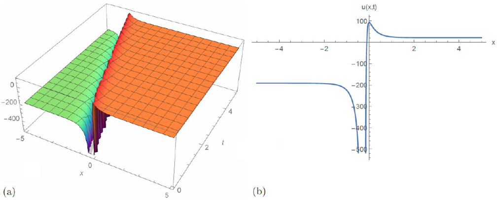
In this section, we present 3-dimensional and 2-dimensional surface plots of the chosen exact solutions obtained by the NEDAM. The plots are presented for several values of α, β, σ, A, p, q, k, w, l, m coefficients and μ, the conformable fractional derivative. While Figs. 1, 2, and 3 represent periodic wave solutions for u 1(x, t), u 2(x, t), u 4(x, t), Fig. 4 is an example for solitary wave solution u 37(x, t) for x ∈ [-5, 5] and t ∈ [0, 5]. As seen, the double periodic solutions are deteriorated to solitary wave solutions and the amplitude goes to infinity.

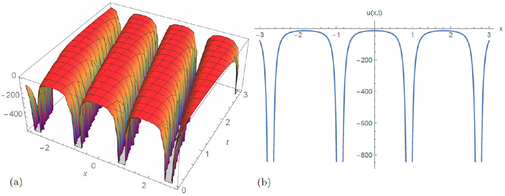
Figure 1 3D and 2D simulation of solution u 1(x; t) for α = 2; β = 3; σ = 1:5; A = e; p = 0:9; q = 0:9; k = 2; w = 1, and μ = 0:90: 

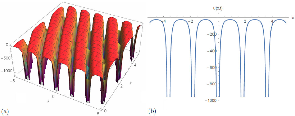
Figure 2 3D and 2D simulation of solution u 2(x; t) for α = 3; β = 3; σ = 1; A = e; p = 0:95; q = 0:95; k = 2; w = 2, and μ = 0:90: 

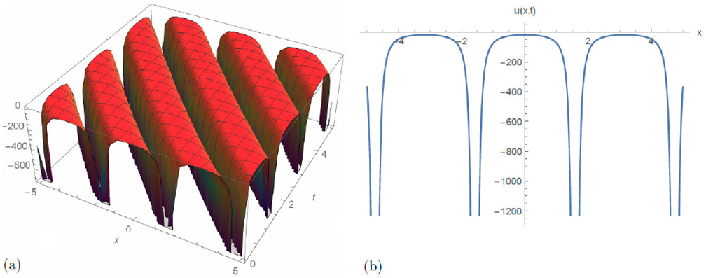
Figure 3 3D and 2D simulation of solution u 2(x; t) for α = 3; β = 3; σ = 1; A = e; p = 0:95; q = 0:95; k = 2; w = 2, and μ = 0:90: 

Figure 4 3D and 2D simulation of solution u 4(x; t) for σ = 1; α = 2; β = 2; A = 2:7; p = 1; q = 1; k = 1; w = 2, and μ = 0:90: 

6. Conclusion

In this study, the new extended direct algebraic method (NEDAM) has been successfully applied to time-fractional SRLW partial differential equation, which arises in long water flow models. The traveling wave transform is used to reduce the equation to integer order ordinary differential equation and with the aid of mathematical software Mathematica and using the conformable derivative definition, numerous new exact solutions of the equation have been obtained which do not exist in the literature. These solutions include rational, exponential, generalized trigonometric, and generalized hyperbolic function series. Thus, it is shown that the method is very effective and powerful as compared with other existing methods in the literature and could be used for different types of FPDEs arising in different areas of mathematical physics.

References

1. Y. Zhaosheng and L. Jianzhong, Applied Mathematics and Mechanics, 19 (1998) 717. https://doi.org/10.1007/BF02457746 [ Links ]

2. B. Senol, A. Ates, B.B. Alagoz and C. Yeroglu, ISA trans. 53 (2014) 189. https://doi.org/10.1016/j.isatra.2013.09.004 [ Links ]

3. K.B. Oldham, Adv. Eng. Softw. 41 (2010) 9. https://doi.org/10.1016/j.advengsoft.2008.12.012 [ Links ]

4. O. Heaviside, Electromagnetic theory, (Cosimo Inc. 2008) 3. https://doi.org/10.1016/j.advengsoft.2008.12.012 [ Links ]

5. A. Carpinteri and F. Mainardi, Fractals and fractional calculus in continuum mechanics (Springer-Verlag, Vienna, 2014), p. 378. https://doi.org/10.1007/978-3-7091-2664-6 [ Links ]

6. I. Podlubny, Fractional differential equations (Elsevier, 1998) 198. [ Links ]

7. A. Yakar and M.E. Koksal, Abstr. Appl. Anal. 2012 (2012) 267108. https://doi.org/10.1155/2012/267108 [ Links ]

8. D. Baleanu, Y. Ugurlu and B. Kilic, J. Comput. Nonlinear Dynam. 10 (2015) 051016. https://doi.org/10.1115/1.4029254 [ Links ]

9. A. Kurt, O. Tasbozan and D. Baleanu, Opt. Quantum Electron. 49 (2017) 333. https://doi.org/10.1007/s11082-017-1163-8 [ Links ]

10. O. Tasbozan, M. Şenol, A. Kurt and O. Özkan, Ocean Eng., 161 (2018) 62. https://doi.org/10.1016/j.oceaneng.2018.04.075 [ Links ]

11. M. Inc, A.I. Aliyu, A. Yusuf and D. Baleanu, Optik 157 (2018) 267. https://doi.org/10.1016/j.ijleo.2017.11.061 [ Links ]

12. B. Ghanbari and J.F.G. Aguilar, Rev. Mex. Fis. 65 (2019) 503. https://doi.org/10.31349/RevMexFis.65.503 [ Links ]

13. B. Ghanbari, and J.F.G. Aguilar, Rev. Mex. Fis. 65 (2019) 73. https://doi.org/10.31349/RevMexFis.65.73 [ Links ]

14. M.S. Osman and B. Ghanbari, Optik 175 (2018) 328. https://doi.org/10.1016/j.ijleo.2018.08.007 [ Links ]

15. B. Ghanbari, M.S. Osman, and D. Baleanu, Mod. Phys. Lett. A, 34 (2019) 1950155. https://doi.org/10.1142/S0217732319501554 [ Links ]

16. B. Ghanbari, A. Yusuf and D. Baleanu, Adv. Differ. Equ. 2019 (2019) 49. https://doi.org/10.1186/s13662-019-1964-0 [ Links ]

17. M.S. Osman, B. Ghanbari and J.A.T. Machado, Eur. Phys. J. Plus, 134 (2019) 20. https://doi.org/10.1140/epjp/i2019-12442-4 [ Links ]

18. B. Ghanbari and M. Inc, Eur. Phys. J. Plus, 133 (2018) 142. https://doi.org/10.1140/epjp/i2018-11984-1 [ Links ]

19. B. Ghanbari and N. Raza, Mod. Phys. Lett. B 33 (2019) 1950018. https://doi.org/10.1142/S0217984919500180 [ Links ]

20. Y. Cenesiz, D. Baleanu, A. Kurt, and O. Tasbozan, Waves Random Complex Media 27 (2017) 103. https://doi.org/10.1080/17455030.2016.1205237 [ Links ]

21. M. Eslami and H. Rezazadeh, Calcolo 53 (2016) 475. https://doi.org/10.1007/s10092-015-0158-8 [ Links ]

22. K. Hosseini, P. Mayeli, and R. Ansari, Optik 130 (2017) 737. https://doi.org/10.1016/j.ijleo.2016.10.136 [ Links ]

23. D. Kumar, A. R. Seadawy and A. K. Joardar, Chin. J. Phys., 56 (2018) 75. https://doi.org/10.1016/j.cjph.2017.11.020 [ Links ]

24. M.S. Hashemi and M. Bayram, Rev. Mex. Fis. 65 (2019) 529. https://doi.org/10.31349/RevMexFis.65.529 [ Links ]

25. V.F.M. Delgado, J.F.G. Aguilar and M.A.T. Hernández, Rev. Mex. Fis. 65 (2019) 82. https://doi.org/10.31349/RevMexFis.65.82 [ Links ]

26. R. Khalil, M. Al Horani, A. Yousef and M. Sababheh, J. Comput. Appl. Math., 264 (2014) 65. https://doi.org/10.1016/j.cam.2014.01.002 [ Links ]

27. A. Atangana, D. Baleanu and A. Alsaedi, Open Math. 13 (2015) 889. https://doi.org/10.1515/math-2015-0081 [ Links ]

28. O. Tasbozan, Y. Cenesiz and A. Kurt, Eur. Phys. J. Plus, 131 (2016) 244. https://doi.org/10.1140/epjp/i2016-16244-x [ Links ]

29. T. Abdeljawad, J. Comput. Appl. Math. 279 (2015) 57. https://doi.org/10.1016/j.cam.2014.10.016 [ Links ]

30. S. Ahmadian and M. T. Darvishi, Optik, 127 (2016) 10697. https://doi.org/10.1016/j.ijleo.2016.08.085 [ Links ]

31. A. Akbulut, M. Kaplan and A. Bekir, Int. J. Nonlinear Sci. Numer. Simul. 17 (2016) 413. https://doi.org/10.1515/ijnsns-2016-0023 [ Links ]

32. K.K. Ali, R.I. Nuruddeen and K.R. Raslan, Chaos Solitons Fractals, 106 (2018) 304. https://doi.org/10.1016/j.chaos.2017.11.038 [ Links ]

33. J.F. Alzaidy, Am. J. Math. Anal. 1 (2013) 14. http://www.sciepub.com/journal/AJMALinks ]

34. S.M. Ege, and E. Misirli, Romanian J. Math.Comput. Sci. 6 (2016) 106. http://www.rjm-cs.roLinks ]

35. A. Korkmaz, O.E. Hepson, K. Hosseini, H. Rezazadeh and M. Eslami, J. King Saud Uni. Sci. 32 (2020) 567. https://doi.org/10.1016/j.jksus.2018.08.013 [ Links ]

36. S.T. Mohyud-Din and S. Bibi, Opt. Quantum Electron. 49 (2017) 64. https://doi.org/10.1007/s11082-017-0895-9 [ Links ]

37. M. Shakeel and S.T. Mohyud-Din, Adv. Trends Math. 2 (2015) 1. https://doi.org/10.18052/www.scipress.com/ATMath.2.1 [ Links ]

38. A. Sonmezoglu, Adv. Math. Phys., 2015 (2015) 1. https://doi.org/10.1155/2015/567842 [ Links ]

39. E.H. Zahran, Int. J. Comput. Appl. 109 (2015) 12. https://doi.org/10.5120/19247-0619 [ Links ]

40. F. Xu, Phys. Lett. A, 372 (2008) 252. https://doi.org/10.1016/j.physleta.2007.07.035 [ Links ]

41. E.M. Zayed, Y.A. Amer and R.M. Shohib, Int. J. Eng. Appl. Sci. 4 (2014) 17. http://www.eaas-journal.orgLinks ]

42. E.M. Zayed, Y.A. Amer and R.M. Shohib, Ital. J. Pure Appl. Math, 34 (2015) 463. http://ijpam.uniud.itLinks ]

43. H. Rezazadeh, H. Tariq, M. Eslami, M. Mirzazadeh and Q. Zhou, Chinese Journal of Physics, 56 (2018) 2805. https://doi.org/10.1016/j.cjph.2018.08.001 [ Links ]

44. H. Rezazadeh Optik, 172 (2018) 545. https://doi.org/10.1016/j.ijleo.2018.06.111 [ Links ]

45. H. Rezazadeh, Optik 167 (2018) 218. https://doi.org/10.1016/j.ijleo.2018.04.026 [ Links ]

46. W. Malfliet, American Journal of Physics, 60 (1992) 650. https://doi.org/10.1119/1.17120 [ Links ]

Received: November 18, 2019; Accepted: December 20, 2019

Creative Commons License This is an open-access article distributed under the terms of the Creative Commons Attribution License