


 nueva página del texto (beta)
 Inglés (pdf)
 Artículo en XML
 Referencias del artículo
 Enviar artículo por email
 Citado por SciELO
  Similares en
SciELO
Similares en
SciELO 
 Permalink
1. Introduction
The subject of fractional calculus has a long history dating back to the time when the derivative of order 1/2 was described by Leibniz to L’ Hopital in 1695 [1]. In recent years, fractional calculus has found its way in many areas of applied sciences and engineering, and it has been demonstrated that modeling physical systems using fractional calculus is more accurate than using integer calculus. This is because the behaviour of many physical phenomena depends on the previous time history (see Mohammed et al. [2]).
There are several works on fractional calculus, such as the work of Eze and Oyesanya [3], who presented a fractional order climate model in the Pacific Ocean. Eze and Oyesanya [4] also used a fractional model to study the impact of climate change with dominant earth’s fluctuations. In the work of Mohamed and Amnah [5], a numerical technique for the estimation of stochastic response of the Duffing oscillator with fractional order damping driven by white noise excitation was introduced. An approach for solving fractional differential equations using exp-function and (G’/G)-expansion method was used in Ahmet et al. [6]. Djurdjica et al. [7] constructed the exact and the approximate solutions of Fuzzy fractional differential equation in the sense of Caputo Hukuhara differentiability with a Fuzzy condition. Rand et al. [8] reviewed the concept of fractional derivatives and derived expressions for the transition curves. Yin [9] applied Legendre spectralcollocation method to obtain approximate solutions of nonlinear multi-order fractional differential equations. Pranay and Rubayyi [10] used Smudu transform and the variable method to solve differential equations and fractional differential equations related to entropy wavelets.
In this work, we shall propose a simple analytical method (which is an elegant combination of a well known methods; perturbation and Laplace methods) to solve non-linear and non-homogeneous fractional differential equations since Laplace method alone is incapable of handling non-linear and non-homogeneous fractional differential equations because of non-linear terms. In particular, we shall analyze the fractional Duffing oscillator using the proposed method.
The advantage of this proposed method over others such as, Adomian decomposition, Modified Laplace decomposition method, (G’/G)-expansion, Homotopy perturbation, Yang-Laplace, and so on, is its ability to handle the complicated non-homogeneous part of the fractional differential equation.
2. Definition of special functions in fractional calculus
In this section, we shall give some definitions related to Caputo’s fractional derivative since in Caputo definition of Fractional calculus, we can find a link between what is possible and what is practical. We shall therefore note that our concentration in this presentation will be on Caputo fractional derivative.
Definition 2.1 The Left Caputo Fractional Derivative (LCFD) is defined by [11]
where 0 < q − 1 ≤ α < q ,q ∈ Z +, t 0 is the initial time and Γ(.) is the Gamma function.
Definition 2.2 The Right Caputo Fractional Derivative (RCFD) is defined by [11]
where 0 < q − 1 ≤ α < q ,q ∈ Z +, t 0 is the initial time and Γ(.) is the Gamma function.
Definition 2.3 In a Caputo’s sense, the Laplace transform of fractional derivative with order α for a function u(t) is defined by [12]
Definition 2.4 A two parameter function of the Mittag-Leffler (ML) function is defined by
Definition 2.5 The Laplace transform of ML is given by
3. Methodology of the new solution
Now we propose a simple analytical method for solving nonlinear and non-homogeneous fractional differential equations.
To show the basic idea, let us consider the following fractional differential equation:
with intial conditions
where α = [α
1
,α
2
,...,α
n
], β = [β
1
,β
2
,...,β
n
], indicating fractional orders,
Now, we seek to find the solution in order of ∈, say, power of ∈, that is
We now substitute Eqs. (8) into (6) and (7) and carry out the expansions in terms of the small parameter to obtain the following system of linear fractional differential equations:
with intial conditions
where A is a linear operator.
Therefore, the linear fractional differential Eqs. (9) with initial conditions (10) can now be solved in succession using the fractional differential property of Laplace transform in Eq. (3).
Note that in this method, it is necessary to express the fractional differential equation in dimensionless form to bring out the important dimensionless parameter that govern the behaviour of the system.
To demostrate the effectiveness of the proposed method, let us consider the general form of Duffing equation which is given by [13,14]:
with initial conditions
Now, we shall use the proposed fractional operator in Rosales et al. [15,16] to construct a fractional Duffing oscillator. The idea is to introduce an auxiliary parameter (σ) in the system such that this σ must have a dimension in seconds and consistent with the dimension of the ordinary derivative operator. In the work [16], the parameter σ was introduced for the first time, but its geometric interpretation is not treated. After that, this method was applied in the work [15].
Now using the proposed idea, we have
Using (13), the Eq. (11) can be written in terms of fractional time derivatives as:
Now expressing Eq. (14) in dimensionless form, we take initial displacement x
0
where u and t denote dimensionless quantities.
Therefore, substituting (15) in (14), we have
with initial conditions
where
and
The function ω(δt) is a slowly varying (sv) function which is defined as follows:
Definition 3.1 (see R. Bojanic and E. Seneta [17]): ω is a sv function if it is a real-valued, positive, and measurable function on [A,∞), A > 0 , and if
for every δ > 0.
Therefore, we shall choose ω(δt) = 1 − e −δt , ( 0 < δ << 1) and let ω to be a sv function of t with right hand derivatives of all orders at t = 0, such that ω(0) = 0 and |ω| << 1,
The symbols
Now let
so that
and
From Eqs. (20) and (21) we have, respectively,
and
Now using Eq. (26), we have
and
where
Substituting Eqs. (27) and (28) in Eq. (16), we have
We now assume the solution in the following asymptotic series:
Equating equations of order (∈ i ,δ j ) in Eq. (29) using the series (30), we obtain the following linear fractional differential equations:
etc.
Now using the scales Eqs. (19)-(21) and the series Eq. (30) on initial conditions Eq. (17), we obtain the following initial conditions:
etc.
Now, using the fractional differential property of Laplace transform in Eq. (3), we can easly obtain the values of U ij as:
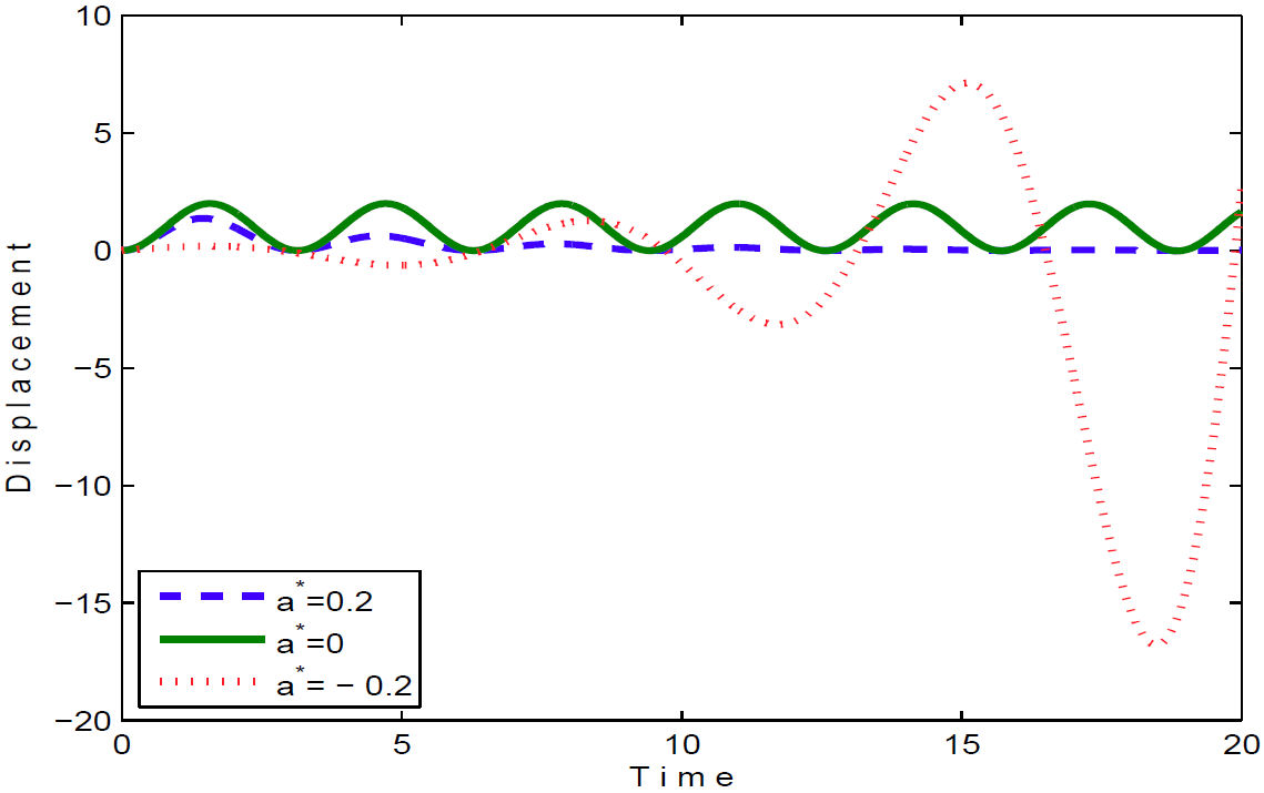
Now, if we substitute the values of U ij which are given in Eq. (43) into Eq. (30) and plot the displacement-time graphs, then we obtain Figs. 1 and 2.
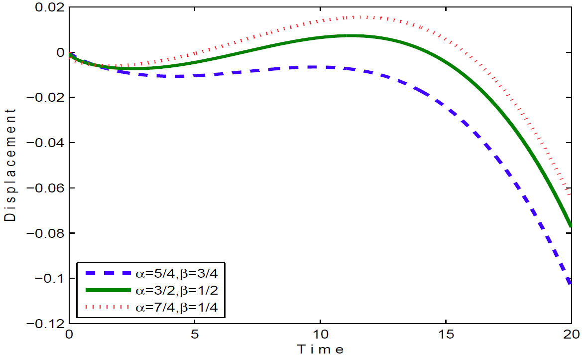
FIGURE 1 Solution in fractional orders, (α = 5/4, β = 3/4), (α = 3/2, β = (1/2) and (α = 7/4, β = 1/4):
4. Conclusion
In this paper, a new analytical method to solve non-linear and non-homogeneous fractional differential equations was proposed. This new analytical method is an elegant combination of well known methods; perturbation and Laplace methods. This method was used to analyze the fractional Duffing oscillator. The performance of this method is reliable, effective and can be used to solve other non-linear and nonhomogeneous fractional differential equations; it can also be extended to solve non-linear and non-homogeneous partial fractional differential equations.

