nueva página del texto (beta)
 Inglés (pdf)
 Artículo en XML
 Referencias del artículo
 Enviar artículo por email
 Citado por SciELO
  Similares en
SciELO
Similares en
SciELO 
 Permalink
1. Introduction
1.1 Renewables investment is stagnating
Driven by falling costs and economic attractiveness, renewables1 are at the heart of the world’s energy transition. Renewables are an economical answer to address climate change and energy security issues (IRENA, 2016). They are a fundamental part of the UN 2030 Sustainable Development Goals. Although there is high optimism regarding the continued deployment of renewable energy technologies, investments have started to slow down. After peaking in 2015, investments in renewable energy decreased from USD 318.8 billion to USD 288.3 billion in 2018 (IRENA, 2021). Some researchers note that renewables face a significant and unique problem for their future deployment: as penetration grows, its value to the system decreases. A problem better explained by the phrase: “the next PV panel will only generate more lunch-time electricity when dinner-time electricity is what is really needed” (Sivaram, 2018).
1.2 Renewable energy decreasing value
The decrease in the value of renewables has been investigated with academic rigour. In competitive electricity markets2, the amount of the decrease of the value can be measured in monetary units per energy units (e.g. $/MWh). Academic studies around the world have found that renewables depress electricity prices (“Price”) given their low marginal costs. The extent up to which renewables depress Price depends upon characteristics of the power market (i.e. demand patterns and misalignments with supply, flexibility of the system and the current energy-mix). The intermittency characteristic of renewables and the fact that electricity physical laws determine that electricity must be supplied at the moment it is produced, aggravate the problem3. Some studies have found that the value of renewables, measured by the price renewables received for the electricity generated, is already below the average electricity value. Most of these studies have been made in mature markets like in Europe or USA, in a context with stagnated or decreasing electricity demand, energy-efficiency improvements, demand patterns sometimes aligned with little sunshine and cold winter weather or where renewables already account for a large share of the generation mix (see: Sensfuss, Ragwitx, Geneoese, 2008; Gelabert, Labandeira & Linares 2011, Würzburg, Labandeira & Linares 2013; Clò, Cataldi & Zoppoli 2015; López Prol, Steininger & Ziberman 2020).
1.3 Geographic context: Young Mexican Wholesale Electricity Market
For the most part of the XX century and the first decade of the XXI century, the power sector in Mexico was restricted and included very little participation from the private sector. There were no electricity markets, and prices and tariffs were set by the Ministry of Finance (Alpisar-Castro & Rodríguez-Monroy, 2016). The 2013 Energy Reform modified several laws to allow the participation of private firms in the energy sector as well as the creation of a wholesale electricity market (see: KPMG, 2016).
Although the implementation policy is being revised4, there has been an increase in renewable electricity generation. In 2012, at the time of the Energy Reform, clean power5 in Mexico accounted for 15% of generation. In 2018 23.2% of electricity was generated by clean technologies, 4% was from wind power (“Wind”) and photovoltaic (“PV”) and 942MW of Wind and 1,316MW of PV were added to the market mix (SENER, 2019).
Throughout that time, most of the renewable generation projects were developed around long-term Power Purchase Agreements (“PPAs”) with high quality off-takers (i.e. an investment-grade commercial or industrial client that would signed a 15 to 20 years contract to buy electricity from the generator at a fixed price). Some of them with CFE, the State-owned electric utility as the result of contract auctions. The PPAs helped these projects as an anchor to find financing and this sort of structure, with most of the revenues coming from PPAs, became mainstream within banks and equity investors. More recently, high-quality PPAs have become scarce as most investment-grade off-takers have secured their electricity needs and State contract auctions have stopped (Bancomext, GIZ, KfW, 2019).
This context has pushed projects to the wholesale electricity market, becoming increasingly important that financing parties have a clear understanding of the market and the pricing mechanisms to make proper assessments of projects with market risks.
1.4 Objective
This research aims to find the depressing effect on the electricity price renewables have in the Mexican wholesale electricity market (i.e. renewables “merit-order” effect; the “MOE”) and their true market value (i.e. the price received for the energy generated compared against the price received by other power sources; “MV”), following the creation of the wholesale electricity market. The objective is to close a gap in the literature about a power market where i) demand is not in stagnation but is increasing, ii) demand is theoretically aligned with warm weather conditions and iii) where renewables do not yet account for a large share of generation (characteristics of the Mexican electricity market and many other markets of which no academic research has been done). Furthermore, the power market in Mexico has only been operating freely since the end of January of 2016 and there is not yet a study that portrays the value of renewables in that market during this time. Finally, this research aims to be significant for debt and equity investors in the Mexico power sector as the need to finance renewable projects with market-risks and without PPAs arises, as well as to investors and policymakers in other power markets with similar characteristics.
2. Literature review: Integration of renewable power in the wholesale electricity-market
2.1 Basis of wholesale electricity-markets
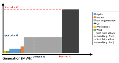
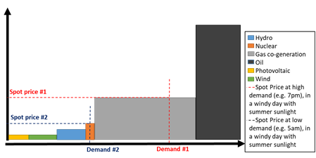
In the short-term markets, the price of settlement is the “spot price” of electricity. The system operator (“SO”) selects the offers based on their price, from cheapest to most expensive (i.e. least-cost dispatching rule). The sell offers theoretically reflects their marginal cost. All dispatchable units (i.e. offers selected by the SO) receive the same Price (for each specific time, space and settlement-time). This means that the last offer to be selected (i.e. the production unit that serves the last unit of the required load6) is the one that sets the Price for all selected units (the “marginal plant”). All generators that are below the intersection with the demand curve are selected to be dispatched and receive the same Price for the amount of power produced. This pricing mechanism is repeated every period, which is a pre-determined time-interval (one hour in the Mexican market).
2.2 Merit-order effect
2.2.1 Theoretical review of the merit-order effect
Jensen and Skytte (2002) introduce the decreasing-effect of renewable power in electricity prices. Theoretically, the increase in intermittent non-dispatchable renewable energy (i.e. sources whose output cannot be control as in the case of wind and solar) generation should reduce the electricity price given its close-to-zero marginal cost (see: Jensen and Skytte, 2002; Sensfuss, Ragwitx, Geneoese, 2008; Nicolosi & Fürsch, 2009). When renewables are generating, they are place at the beginning of the supply stack. This pushes more expensive units out of the intersection with the required demand, therefore the last unit to be selected to meet the required demand is cheaper than in a scenario without renewables. This came to be known as the “merit-order effect”.
2.2.2 Merit-order effect empirical studies - historical data tests
Several empirical studies have been made to test the data with similar approaches. Although results may vary, they consistently find a MOE.
Woo, Horowitz, Moore & Pacheco (2011) do one of the first empirical-based studies of Texas with data from 2007 to 2010 and explore the effect that Wind has on the market with high frequency observations at 15-min resolution7; they find that 100MWh of Wind reduces Price between US$0.32/MWh and US$1.53/MWh depending on the Texas zone. Gelabert, Labandeira & Linares (2011) study the effect of renewables jointly with cogeneration under a support special regime in Spain from 2005 to 2010; they find that 1GWh increase of generation under the mentioned special regime is associated with a reduction of €1.9/MWh. Welisch, Ortner & Resch (2016) do the first study for a single regression model that can be applied in several markets and provide a multi-country analysis, with data from Germany, Ireland, France, Belgium, Spain, U.K. and Denmark; their model seems suitable for assessing the MOE in the European context, yet country-specific variables seem to play a role8. Clò, Cataldi & Zoppoli (2015) study the Italian wholesale electricity market from 2005 to 2013 and explore the effect of wind and solar generation independently; they find that 1GWh increase of PV reduces Price by €2.3/MWh while 1GWh increase of Wind reduces Price by €4.2/MWh. These studies consistently find that renewable electricity generation has a negative effect on electricity price (i.e. the MOE).
Several other factors have been found to affect Price. Local electricity demand (i.e. zone load; “Load”) has significant explanatory power over Price. As expected, an increase in demand is related with an increase in price. Even in the same market, different zonal loads may show significant different impacts over Price, although all of them show a positive effect over Price. (see: Woo, Horowitz, Moore & Pacheco 2011, Gelabert, Labandeira & Linares 2011). Given that the electricity markets follow seasonal patterns, most ex-post studies use day-of-the-week and month variables to control for seasonality and these variables have shown to have a large explanatory power of the electricity price (see: Gelabert, Labandeira & Linares 2011, Würzburg, Labandeira & Linares 2013). Demand and seasonality alone can explain up to 50% of the Price (see: Clò, Cataldi & Zoppoli, 2015). Given the “least-cost dispatching rule”, the output of dispatchable power plants is endogenous with Price, yet, their fuel costs are exogenous. The fuel cost of dispatching generators has a positive relationship with Price, nevertheless, the strength of their explanatory power depends on the matrix of the system and the usual marginal plants (see: Woo, Horowitz, Moore & Pacheco 2011, Clò, Cataldi & Zoppoli, 2015). Price is also positively influenced by the price of previous dispatching intervals, whether it’s the previous dispatching interval (see: Woo, Horowitz, Moore & Pacheco 2011) or the Price of a comparable time (see: Welisch, Ortner & Resch 2016). Furthermore, Price has been found to be related with base-load non-dispatchable generation (e.g. nuclear) (see: Woo, Horowitz, Moore & Pacheco 2011) and transmission across markets and borders (i.e. net exports) (see: Würzburg, Labandeira & Linares 2013).
Gelabert, Labandeira & Linares (2011) explore the effect of renewables over prices at different levels of demand (i.e. data sets of different quartiles of demand) and find that the effect is greater when demand is higher. Welisch, Ortner & Resch (2016) add squared-terms of demand and renewable generation to allow for different levels of price elasticity, although they find neither of them to be economically or statistically significant. López Prol, Steininger & Ziberman (2020) explore non-linearity through both methods (different data sets and quadratic terms) and find relevant results (although their model is more focused on MV - a topic explained in the following sections - and cross cannibalization). These studies have found that at different levels of demand and at different levels of renewables penetration, the MOE may be different (i.e. a non-linear MOE).
A recurrent issue is the different MOE causes and effects between Wind and PV. Luňáčková, Prusa & Janda (2017) find that PV has a slight increasing relationship with Price while the rest of renewable power does have a decreasing effect. Hirth (2013) finds that PV’s MV falls from above the average electricity price to around half of that at a faster rate than Wind’s MV in Europe. A similar conclusion can de derive of López Prol, Steininger & Ziberman (2020)9 with non-linear results in their study in California. Yet, Würzburg, Labandeira & Linares (2013) find no difference between the MOE of Wind and PV. Although both technologies are intermittent in nature, their production profile varies significantly. In one year, around 80% of PV is produced in 26% of the time, whereas 80% of Wind is produced in 47% of the time (Hirth, 2015). The implication is that the nature of Wind’s MOE is different from that of PV’s. Depending on demand patterns, whether they are aligned with warm weather, air conditioners during the day, long-sunshine days, or with cold weather, heating systems during the night, and few hours of sunshine, PV and Wind will have different MOE (MIT Energy Initiative, 2015). PV generation may not be enough to push the marginal plants out of the dispatching curve, therefore not causing a MOE (Luňáčková, Průša, & Janda, 2017). Wind may benefit from PV due to pronounced ramping costs when the sun goes down, therefore wind may not reflect a MOE (López Prol, Steininger, & Zilberman, 2020).
These empirical studies are the base of the methodology of this research, although several other studies have found a conclusive MOE using other empirical model specifications (see: Sáenz de Miera et al. 2008), studying the interaction with climate-change/energy-related policies (see: Weigt, 2009; Linares et al., 2008), as well as in simulation-based studies (see: Sensfuss, Ragwitz & Geneoese 2008)10.
A comparison of some of these methodologies is shown in Annex 1.
2.3 Market-value of renewable power
2.3.1 Theoretical review of the real market-value of renewables
Hirth (2013) and Hirth (2015) explain the MV of electricity as the average spot price in the respective market, given in currency over electricity units (e.g. €/MWh), received by the technology or power plant in question. This definition implies that there’s a different MV for each power plant depending on their supply and demand interaction context. Hirth (2015) addresses the issue of the real MV of renewable energy on the basis that it is “not correct to assume that 1) the average price of electricity is the same as the average price of electricity from renewable sources, or 2) the price that different technologies receive is identical”. Furthermore, he introduced the “value-factor” concept as a tool to compare MV of a specific technology or power plant against the average spot MK (the “VF”).
2.3.2 Renewables real MK empirical evidence
Based on the MOE, empirical studies have been made that consistently show that the MV of renewables is below the average MV.
Hirth (2015) does an empirical analysis of the true MV of solar in Germany. He finds that PV’s VF decreases between 2.2% and 5.5% per 1% increase of market-share (depending on the method). Further, the results show that at low penetration rates, PV’s MV is greater than the average electricity MV in Germany, but that it rapidly decreases below the average when it’s market-share increases. This decrease is much steeper for PV than for Wind. Welisch, Ortner & Resch (2016) find the MK of wind electricity to be 90% of the average MK in Germany in 2012, whereas the MV of PV was above the average MK, at 106% of the average. López Prol, Steininger & Ziberman (2020) find that the VF of solar energy11 decreases 4.1% per 1% increase in penetration and the VF of Wind decreases 0.9% per 1% increase in penetration. Interestingly, at different levels of penetration, whereas penetration of wind causes that both the value of wind and solar decrease, the penetration of solar causes a decrease on its own but not on wind’s value, which may be due to their opposite generation patterns (i.e. solar generation concentrated in day-time and wind generation distributed across all 24 hours) and the ramp-up of gas turbines at night-fall that causes a price spike.
These studies add to the evidence of the different nature of the MOE between Wind and PV and its relevance at different levels of demand and generation.
3. Methodology of this research
3.1 Merit-order effect empirical research methodology
For the MOE estimation in the Mexican wholesale electricity-market, I use different specifications of a multivariate linear regression model (based on the methodologies compared in Annex 1). The multivariate linear regression methodology has proved effective to understand the historic drivers of electricity price in the before mentioned studies and the variables chosen for each model specification have proved to be significant within those studies.
Where:
P = Price
Renew = Wind Electricity + PV Electricity
Wind = Wind Electricity
PV = PV Electricity
Load = Demand of Electricity
ControlVars = control variables (i.e. Gas Price, Lagged Electricity Price and trend)
x = subindex that refers to different coefficient estimators of the different control variables.
dummies = seasonality control variables (i.e. week-day, month and holidays)
z = subindex that refers to the different coefficient estimators of the different “dummies”
t = load-time
Price is the dependent variable. It is called Local Marginal Price (“PML” for its Spanish acronym) in the Mexican Wholesale Market. It is the price of the day-ahead market. The day-ahead market was chosen over the hour-ahead and the real-time markets given that it represents a larger share of the trading volume (see: Gelabert, Labandeira & Linares 2011). Price moves across the space dimension (i.e. node of Load - see: Hirth, 2015), to deal with this, the average of price of each node is taken. P is the average wholesale price of all nodes of the National Interconnected System (“SIN” for its Spanish acronym, that is the electric system that comprises ~99% of total Load of the Mexican electric system), of the day-ahead market, given in Mexican Peso over MWh ($/MWh) at a given time12t.
Renewable electricity generation is the explanatory variable of main interest. The main aim of this research is to find how much the price is affected by renewable energy. The data is taken from the day-ahead forecasts composed by the SO, based on information provided by the generators. The data shows the forecast of intermittent non-dispatchable generation separated by source (i.e. PV and Wind). Renew is the sum of the day-ahead forecast of generation of all renewable generators of the SIN (separately by Wind and PV or jointly depending on the model specification) given in MWh13.
Demand is another explanatory variable. Basic economic theory explains that when demand grows price increases, and this has proved to hold true in other studies. Load is the sum of the day-ahead forecast of demand of all nodes of the SIN, given in MWh14.
Natural gas price, lagged electricity price and a trend variable are used as control variables since the price of other energy goods and the electricity price of the previous day are valuable indicators of the electricity price (see: Woo, Horowitz, Moore & Pacheco, 2011; Welisch, Ortner & Resch, 2016), although the interpretation of these variables is beyond the scope of this research. In the Mexican wholesale electricity market, more than 80% of power is generated by fossil fuels, and natural gas represents more than 50% of the fuels used for conventional power generation (CENACE, 2017), while gasoline represents 21% and diesel 20%. Since gasoline and diesel data were not available at the needed frequency, and both products are subsidized, natural gas was used as the only control variable for other energy goods. The variable used as gas price is the average natural gas price published by PEMEX (the national government-owned Oil & Gas company) of the previous day (to deal with the forecast nature of the day-ahead market)15 across all different distribution zones and injection points16, given in MXN/GJ. The variable used as lagged electricity price is a 24-hour lag of the electricity price variable P.
Consistently with the literature, monthly, weekly and holiday dummies are used to control for seasonal and weekly demand patterns.
3.2 Data selection and presentation
The period chosen for this study is the period from January 1st, 2017 to December 31st, 201917. These are the first three complete years that the Mexican wholesale electricity market has been operating. Data is in hourly resolution and variables are in levels. Finally, the explanatory variables should match the characteristics of the day-ahead price, therefore the explanatory variables are the day-ahead forecast (except for gas price).
3.3 Econometric review and limitations
Following Gelabert, Labandeira & Linares (2011) example, a variation of the main regression was made using first differences instead of levels that proved not to be a good fit for the data (i.e. R2 = 0.132).
Following Welisch, Ortner & Resch (2016) example, a regression using exports of electricity was tested that proved not to be either economically or statistically significant (the SIN is not a significantly interconnected system, less than 0.01% of Load is exported).
Missing variables are a limitation. CENACE notes that the implied heat rate, the availability of natural gas in the southwest of Mexico, and the saturation of the nodes and congestion of the system, are all determinants of the PML. Although these variables remain in the error term (i.e., εt), a lot of the information they provide is captured through other explanatory variables via collinearity.
To test for the normality of the residuals, a graphic test was used (results showed a normal distribution of the residuals). To test for heteroskedasticity, a Breusch-Pagan test is used (results showed heteroskedasticity in the residuals, i.e., the null hypothesis of constant variance was rejected). To test for serial correlation a Durbin-Watson test is used (results showed positive autocorrelation, i.e., DB test = 0.36). Further, a Breusch-Godfrey test was used (results showed the null hypothesis of no autocorrelation was rejected). The estimators of the regression aim to be asymptotic-valid. The assumptions are as follows: i) the time series is linear in parameters; ii) there is no perfect correlation within the variables, nor very high collinearity; iii) the time series is stationary; iv) there is no strict exogeneity; v) there is weak stationarity (i.e., covariance stationarity: their expected value, variance and covariance are constant over time); vi) the time series is weakly dependent (i.e. observations can be related as long as the relation is weaker when they are further apart in the sequence, therefore, with a large sample, we get the complete picture of the relation of the variables). To deal with heteroscedasticity problems and autocorrelation, serial-correlation-robust standard errors are computed and reported in the results to test the probability that the estimators are zero. The estimators of the regression cannot claim causality as the variables are not strictly exogenous nor all the classical assumptions of the Gauss-Markov Theorem are met to claim they are the best linear unbiased estimators. Nevertheless, given all the assumptions and tests mentioned, the estimators are consistent, tending to the real value and statistically significant.
3.4 MV of renewables methodology
As in Welisch, Ortner & Resch (2016), I compute the MV of renewables. Following Hirth (2015), comparing that figure with the average electricity price is of the interest of this research.
Where:
h = load-time
t = technology
generation = production of respective technology
load = demand in the wholesale electricity market
price = wholesale electricity-price at respective load-time
The amount of renewable generation is multiplied by the electricity price at the respective hour it was generated. That process is repeated for every hour and every day of the period and sum altogether. This yields the true total value of the renewable generated energy in the period. That figure is then divided by the sum of all renewable generation of every hour of every day. This yields a generation-weighted average Price received by renewables (i.e. its MV). That figure in then contrasted with the load-weighted average Price of the market (the Wholesale MV or the Load’s MV)18 to yield a VF of renewable electricity. This is made for both Wind and PV jointly as well as separately.
Furthermore, I conducted a scenario analysis expanding the penetration of renewables to see how it would affect their MV (a similar approach used by Jain & Shrimali, 2022).
4. Data presentation of the Mexican wholesale electricity-market
The summary statistics are presented in the following table. Correlation statistics and data graphs are presented in Annex 2.
Table 1 Summary Statistics
| Summary Statistics | |||||||
|---|---|---|---|---|---|---|---|
| Variable | mean | sd | p25 | p50 | p75 | min | max |
| Price (MXN$/MWh) | 1357.26 | 669.86 | 866.52 | 1242.60 | 1694.03 | 0.00 | 7905.48 |
| Load (MWh) | 33838.53 | 4418.83 | 30747.14 | 33925.28 | 36975.00 | 18686.03 | 47245.72 |
| Gas Price (US$/GJ) | 3.26 | 0.57 | 2.96 | 3.23 | 3.43 | 2.26 | 8.19 |
| Wind Electricity (MWh) | 1465.38 | 690.38 | 874.73 | 1449.22 | 2012.29 | 125.12 | 4011.32 |
| PV (MWh) | 393.99 | 761.56 | 0.07 | 22.21 | 341.67 | 0.00 | 3301.88 |
| Renewable Electricity (MWh) | 1859.36 | 1108.03 | 1005.18 | 1713.27 | 2336.24 | 158.00 | 6398.36 |
5. Analysis and interpretation
5.1 Merit-Order effect empirical analysis of the Mexican wholesale electricity-market
Table 2 Merit-Order Effect Linear Regression Coefficients
| (1) | (2) | |
|---|---|---|
| Renewables | -0.0986*** | |
| (0.00288) | ||
| Wind | -0.144*** | |
| (0.00435) | ||
| PV | -0.0625*** | |
| (0.00405) | ||
| Load | 0.0664*** | 0.0648*** |
| (0.00112) | (0.00112) | |
| Gas Price 24h Price Lag | 146.6*** | 150.8*** |
| (5.623) | (5.620) | |
| 0.495*** | 0.495*** | |
| (0.00844) | (0.00841) | |
| Weekly dummies | ✔ | ✔ |
| Monthly dummies | ✔ | ✔ |
| Holiday dummies | ✔ | ✔ |
| Trend | ✔ | ✔ |
| _cons | -2069.3*** | -1968.1*** |
| (35.58) | (35.72) | |
| # of observations | 25771 | 25771 |
| adj. R-sq | 0.667 | 0.670 |
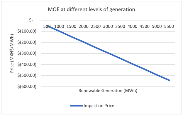
Table 2 presents the results of the MOE empirical analysis. The first model (equation 1) is the classic MOE linear regression model. As expected renewable electricity generation is related with a decrease in electricity price. Based on model 1, renewables show a negative and statistically significant MOE of -MXN$0.10 per MWh. On average, renewables seem to explain a decrease of MXN$183.33/MWh, holding all other variables constant. That is the mean MOE in the day-ahead Mexican wholesale electricity market. To put it in perspective, the average MOE is 13.51% of the average price.19 Given the different nature of Wind and PV, model 2 portrays the MOE of Wind and PV separately (equation 2). The different MOE between these technologies is both economic and statistically significant20. On average, Wind seams to explain a MXN$211.01/MWh decrease in price, 15.5% of the average price, while PV seams to explain a MXN$24.62/MWh decrease in price, just 1.8% of the average price. Overall, the models show a heteroscedasticity robust R2 of 0.66 - 0.67 and the explanatory variables chosen are statistically significant at the 0.01 level. Extending the MOE results based on equations from Table 2 yields the graphs shown in Figures 3, 4 and 5, portraying what would be the impact of the MOE on the electricity price if renewables grew to different levels of penetration.
5.2 Non-linear effects over electricity price
Based on the results of Gelabert, Labandeira & Linares (2011), Würzburg, Labandeira & Linares (2013) and López Prol, Steininger & Ziberman (2020), model 2 was further tested at different levels of demand and at different levels of renewables generation, finding significant difference between the lower and upper quartiles of Load, wind generation and PV generation (Table 3)21.
Table 3 MOE at different levels of demand, wind and PV
| (2) Low Load | (2) High Load | (2) Low Wind | (2) High Wind | (2) Low PV | (2) High PV | |
|---|---|---|---|---|---|---|
| Wind | -0.114*** | -0.170*** | -0.0910*** | -0.121*** | -0.112*** | -0.190*** |
| (0.00410) | (0.0115) | (0.00639) | (0.0138) | (0.00444) | (0.00905) | |
| PV | -0.0286*** | -0.0389*** | -0.0461*** | -0.0323*** | 0.109** | -0.117*** |
| (0.00461) | (0.00742) | (0.00523) | (0.00494) | (0.0453) | (0.00865) | |
| Load | 0.0601*** | 0.0830*** | 0.0709*** | 0.0555*** | 0.0587*** | 0.0726*** |
| (0.00111) | (0.00512) | (0.00138) | (0.00164) | (0.00120) | (0.00387) | |
| Gas Price | 115.1*** | 323.7*** | 144.5*** | 139.1*** | 103.2*** | 162.8*** |
| (5.004) | (24.18) | (7.849) | (6.736) | (5.307) | (13.04) | |
| 24h Price Lag | 0.474*** | 0.518*** | 0.509*** | 0.412*** | 0.506*** | 0.427*** |
| (0.00876) | (0.0168) | (0.00987) | (0.0136) | (0.00955) | (0.0190) | |
| Weekly dummies | ✔ | ✔ | ✔ | ✔ | ✔ | ✔ |
| Monthly dummies | ✔ | ✔ | ✔ | ✔ | ✔ | ✔ |
| Holiday dummies | ✔ | ✔ | ✔ | ✔ | ✔ | ✔ |
| Trend | ||||||
| _cons | -1650.6*** | -3231.9*** | -2125.4*** | -1485.6*** | -1587.8*** | -1954.1*** |
| (33.11) | (203.8) | (47.82) | (56.10) | (35.56) | (102.6) | |
| # of observations | 19257 | 6512 | 19416 | 6355 | 19348 | 6423 |
| adj. R-sq | 0.651 | 0.465 | 0.648 | 0.703 | 0.669 | 0.681 |
| Standard errors in parentheses | ||||||
| "*"=p<0.10 "**"=p<0.05 "***"=p<0.01 | ||||||
Following with these findings, quadratic forms of the variables were included in model 3. Contrastingly with previous research, the non-linear effect of Load and renewable generation proved to be statistically significant. Nevertheless, including these variables in the model undermines the explanatory power of the linear form of wind electricity and demand (but not that of PV, explained in the following sections), therefore another variation of the model was tested based on equation 7 (Table 4).
Table 4 Non-linear MOE equation 7
| (3) | (7) | |
|---|---|---|
| Wind | -0.0212 | |
| (0.0159) | ||
| Wind2 | -0.0000409*** | -0.0000472*** |
| (0.00000489) | (0.00000133) | |
| PV | 0.103*** | 0.103*** |
| (0.0126) | (0.0126) | |
| PV2 | -0.0000688*** | -0.0000685*** |
| (0.00000492) | (0.00000490) | |
| Load | -0.00579 | |
| (0.00741) | ||
| Load2 | 0.00000105*** | 0.000000963*** |
| (0.000000115) | (1.71e-08) | |
| Gas Price | 138.6*** | 138.3*** |
| (5.353) | (5.360) | |
| 24h Price Lag | 0.478*** | 0.478*** |
| (0.00844) | (0.00840) | |
| Weekly dummies | ✔ | ✔ |
| Monthly dummies | ✔ | ✔ |
| Holiday dummies | ✔ | ✔ |
| Trend | ✔ | ✔ |
| _cons | -823.2*** | -931.0*** |
| (120.8) | (22.67) | |
| # of observations | 25771 | 25771 |
| adj. R-sq | 0.675 | 0.674 |
| Standard errors in parentheses | ||
| "*"=p<0.10 "**"=p<0.05 "***"=p<0.01 | ||
5.2.1 Demand’s non-linear effect
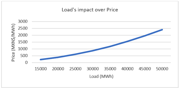
As expected, demand shows a non-linear relationship with Price. There is a significant difference of Load’s coefficient at different quartiles of demand (Table 3)22 and the quadratic form of the variable proved to be statistically significant (Table 4). Although it is beyond the scope of this research, at the lower-end of the curve the impact of demand over price may reflect the fixed-costs of base-load generators whereas the upper-end of the curve results may reflect ramp-up costs and fuel prices of peak-load generators (see: Kwoka & Madjarov, 2007). This last point is further supported by the significant difference in the gas price coefficient at different levels of demand (Table 5). When the system is reaching peak-load, more plants are needed to supply the demand, therefore, peak-load power plants, some of whose marginal costs reflect the gas price, are selected to be dispatched and set the Price.
5.2.2 Non-linear MOE
The difference of the coefficients of renewable energy generation between the lower and upper quartiles of demand implies that the MOE is larger when the system is closer to peak-load and closer to maximum capacity (Table 3). When demand is high, costly peak-load plants are being dispatched and they set the price, therefore a displacement of one of these plants of the intersection of the supply and demand curve via more renewable generation has a greater impact in the electricity price than when renewables are displacing cheaper plants (Gelabert, Labandeira, & Linares, 2011). Wind has a 49.1% higher MOE at the upper demand quartile compared against to the lower quartile, while PV has a 36% higher MOE23.
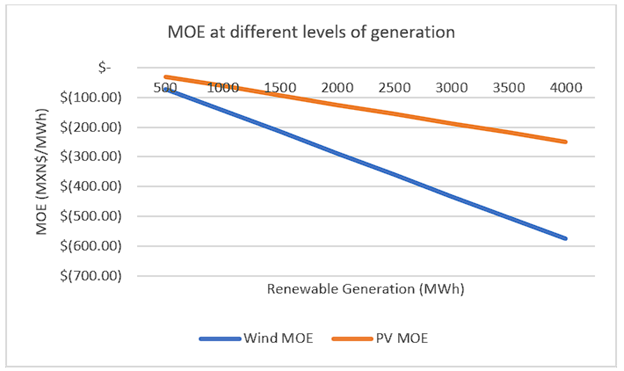
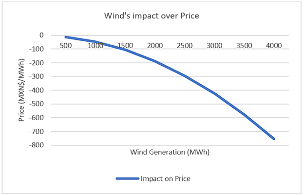
Adding quadratic terms to the model allows to measure how the MOE of Wind and PV increases as their penetration increases, as well as to see that the MOE of Wind and PV is different in nature (Table 4). Based on model 7, on average, Wind seems to explain a decrease of MXN$101.35/MWh, -7.5% of the average price, while PV is related with an increase of MXN$29.95/MWh, 2.2% of the average price24. These figures are significantly different from the linear results of model 2, but, while the average MOE of both Wind and PV is not as large as in the linear specification of the model (model 2), their MOE increases exponentially as penetration increases. At 4000MWh of generation, holding all other variables constant, Wind would produce a MXN$755.2/MWh decrease over the electricity price (Figure 7), significantly larger than MXN$576/MWh based on model 2 (Figure 4). At 3000MWh of generation, PV would produce a MXN$307/MWh decrease over the electricity price (Figure 8), significantly larger than MXN$187.50/MWh based on model 2 (Figure 4).
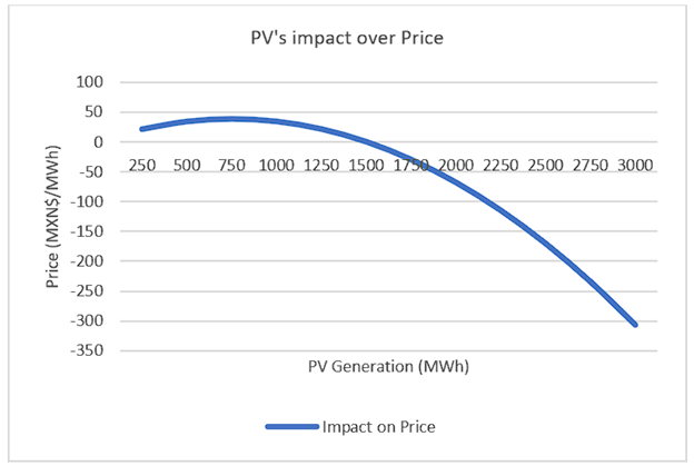
The interpretation of PV’s non-linear MOE is more interesting. At low levels of penetration, PV is related with an increase in price. This is shown both, with a linear model at the lower quartile of PV (Table 4), and by the positive coefficient of the simple term of the variable of model (7) (Table 4). It is only above 751.8MWh of PV that the next MWh of PV has a decreasing effect over Price, and it is only beyond 1503.65MWh that PV is related with a negative MOE (Figure 6). The rational is that when sunshine is low, PV is not enough to push more expensive power plants out of the intersection with demand and bring the Price down. Furthermore, given that sunshine is aligned with demand patterns in Mexico, when PV increases demand often increases more, making it more difficult for PV to show a MOE. It is only beyond a high threshold that PV increases enough to offset the increase in demand and show a MOE (see: Luňáčková, Prusa & Janda, 2017). Beyond this threshold the effect of PV is larger than Wind given that is highly concentrated in time (see: López Prol, Steininger & Ziberman, 2020; Hirth, 2013; MIT Energy Initiative, 2015).
5.3 Renewables MV
The MK (i.e. generation-weighted average price received) of Wind and PV as a whole from 2017 to 2019 was MXN$1,313.31/MWh. The MK of Wind was MXN$1,283.03/MWh, whereas the MK of PV was MXN$1,425.94. Standardizing to the Load’s MV (MXN$1,416.23)25, renewables’ VF is 0.93, 0.90 for wind power and 1.01 for PV.
Expanding the real MV of renewables to the deployment of more renewables, given model 7 MOE, yields the following results:
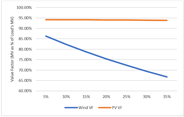
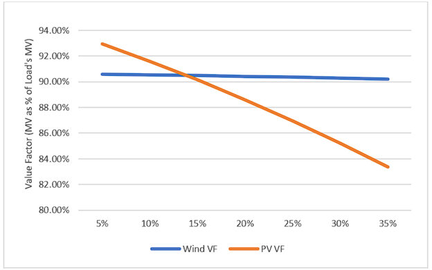
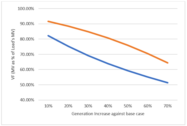
Figures 9, 10 and 11 are interpreted as follows: In each scenario of Wind, PV, or both technologies increase of generation at different levels compared to the 2017-2019 data, given their respective MOE and all other things equal, the changes in Price, Load’s MV, Wind MV and PV MV, yield the graph changes in Wind and PV VF.
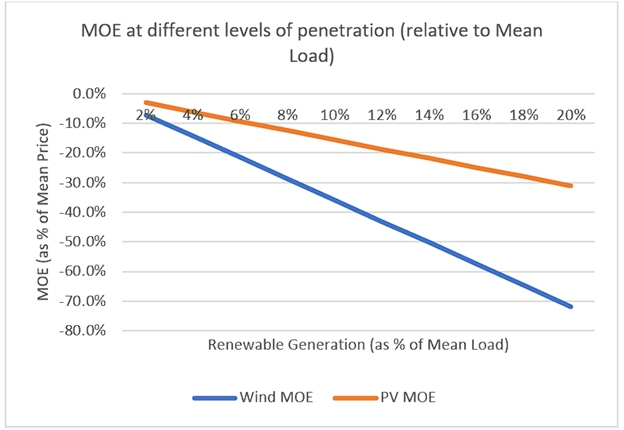
At scenarios with an increase of Wind (figure 7), all things equal, Wind MV rapidly falls below 80% of Load’s MV. At a 35% increase of Wind generation, its MV falls as low as 66.7% of Load’s MV. For perspective, the 35% Wind increase only represents a change of Wind’s share of Load from 4.3% to 5.8%. At a scenario with a 15% increase of PV (figure 8), all things equal, PV MV, originally greater Load Wind MV, falls to 90% of Load’s MV. At a 35% increase of PV, its MV falls below 84% of Load’s MV. For perspective, the 35% PV increase only represents a change of PV’s share of Load from 1.2% to 1.6%. Interestingly, no cross-cannibalization can be observed as in López Prol, Steininger & Ziberman (2020), which is likely due to the fact the Wind and PV generation profiles in Mexico are not as highly contrasting as in Texas (Annex 2). Nevertheless, it should be expected that MOE causes higher-than-expected ramping requirements and that peak Price increase due to scarcity of intermittent generation, therefore benefiting other power plants (see: Sensfuss, Ragwitz & Geneoese, 2008; MIT Energy Initiative, 2015) At a scenario where both Wind and PV increase their generation by 70%, Wind’s MV falls as much as 49% and PV MV falls as much as 35%. For perspective, PV plus Wind represented 5.4% of Load, a 70% increase means renewables would take 9.2% share of Load.
6. Conclusions
These results are in line with previous research and provide new evidence of the non-linear MOE and the different implications of Wind and PV.
As already stablished, all dispatched generators get affected by the MOE, but the extent to which they get affected depends on the hours they overlap with renewable generators. Renewable generators get affect by the MOE with every unit of power they produce and therefore every power unit they produce is less profitable than the previous one (subject to pushing more expensive power plants out of the intersection). Stakeholders should differentiate the average Price from the price received by each power plant. They should expect that costly units are force out of the system and that the average Price drops as a consequence of the deployment of more renewables and the least-cost dispatching rule.
As a rule of thumb, renewables in the Mexican day-ahead wholesale electricity-market show an economically and statistically significant negative relationship between generation and Price of -MXN0.10/MWh per MWh and an average MOE of -MXN183.33/MWh, -13.5% of the average Price. Renewables MV is 93% of the Load’s MV.
Allowing for non-linear interactions and distinguishing between Wind and PV shows that the MOE is largely related with demand levels as well as the penetration of each technology. Wind MOE is much larger at high levels of generation, reaching -MXN755/MWh at 4000MWh of generation. PV MOE is also much greater at high levels of generation, once it’s beyond the 1503MWh threshold, it reaches -MXN307/MWh at 3,000MWh of generation.
7. Further Discussion
The implications of the results of this research are varied. To name a few: i) energy and commodity traders should expect a larger demand for hedging instruments; ii) renewable investors would prefer develop several “small” projects in different Load zones rather that developing one “big” project (or develop a new project rather than increasing the size of an existing one); iii) renewable investors would prefer to develop a new project in a different Load zone instead of increasing the capacity of an existing one; iv) debt financing parties would likely be very cautious with Price forecasts (e.g. limiting their assessments to low Price scenarios); v) debt instruments will likely have a shorter maturity that PPAs-based financing and include market-risk covenants (e.g. cash traps or cash-sweeps linked to Price re-assessments); vi) given the previous points, renewables would find it harder to reach economies of scale via including development costs and financial structuring costs; vi) the system will likely become more flexible, with a growth of flexibility solutions for conventional generators to reduce ramping costs or storage units (either complementary to existing renewables or as independent units).
Most of these impacts are the same impacts that have been seen in more mature markets, although their magnitude will depend on the Mexican market-specific issues (e.g. some Load zones are below the PV MOE threshold therefore investments in renewables would likely continue in the zone).
Although the impact of the current energy policy is beyond the scope of this research, whatever the policy pursued by the Mexican authorities, policymakers should expect that, as the MOE and renewables MK becomes an integral part of investment assessments, investment behavior will change, and they should plan the future of the system accordingly. Further, any subsidy considered for renewables would be better designed if it’s directed to the price received by the generators, that if it’s designed based on CAPEX assumptions given that they wouldn’t capture the missing revenue that these producers would face in a future with high renewable penetration (see: Carvalho Figueiredo & Pereira da Silva, 2019; Sirin & Yilmaz, 2020). These results may serve as a tool to generate mechanisms that alleviate the MOE (e.g. smart-metering, system-interconnection infrastructure)
Further research can expand to the future development of the energy-mix given the MOE and investment decisions based on renewables MV, as well as policies to alleviate the MOE.