


 nueva página del texto (beta)
 Inglés (pdf)
 Artículo en XML
 Referencias del artículo
 Enviar artículo por email
 Citado por SciELO
  Similares en
SciELO
Similares en
SciELO 
 Permalink
1. Introduction
Volatility is an intrinsic phenomenon in the financial markets, which generates uncertainty and significantly affects the prices of financial assets in a given period. Over the years, several models have been developed to measure volatility, but none has been considered optimal to guarantee favorable performance in making predictions (Pilbeam & Langeland, 2015).
It is important to emphasize the differences between historical and implied volatility. Historical volatility is based on historical price series, whereas implied volatility is obtained by observing option prices in the market (D’Agostino et al., 2013). The first models that were developed to measure volatility include the exponentially weighted moving average model, in which historical volatility uses a weighted approach to give increased relevance to more recent measurements (Roberts, 2000). Latané and Rendleman Jr. (1976) proposed a method to calculate implied volatility through the prices of options in the market based on the Black-Scholes (1973) option pricing model put forward by Fischer Black and Myron Scholes in 1973, which uses variables such as price, strike price, volatility, term, and dividends to value financial asset options.
Engle (1982) developed the heteroscedastic conditional autoregressive model, which introduced the concept of a non-constant conditional variance, where information from the recent past is used to predict future volatility. Bollerslev (2001) subsequently proposed the GARCH (1,1) model, which adds a long-term volatility persistence term. In 1996, JP Morgan and Reuters (1996) published the RiskMetrics-Technical Document, which is a set of the main techniques for measuring market risks in portfolios of financial instruments.
Today, the state-of-the-art for the study and prediction of volatility in financial markets uses artificial intelligence tools. An example is the use of long short-term memory artificial neural network models for predicting future volatility in the foreign exchange market, which allows more precision than the traditional methods, but has disadvantages, such as the difficulty in capturing seasonality, including the presence of time lags in the prediction against the target volatility (Liao et al., 2021). Additionally, Olden and Jackson (2002) observe that artificial neural network models are considered “black box” models because they provide little information about the influence of independent variables on the behavior predictive process. Thus, understanding the behavior of the markets beyond the ability to generate a quantitative prediction is difficult.
Despite all these advances in measuring volatility, discrepancies still exist between the models and reality in the markets. The reason is that the implied volatility observed in option premiums in the derivatives market often differs from the volatility calculated by the methods mentioned.
Solís and Muñoz (2018) pointed out that the volatility in the USD/MXN exchange rate has been a constant concern for economic policy in Mexico. In this context, this study aims to investigate whether the VXY and EM-VXY indices have an impact on the implied volatility of three-month at-the-money (ATM) options on the USD/ MXN exchange rate on the Chicago Board Options Exchange (CBOE). With this, the study seeks to contribute to the understanding of volatility in financial markets and its relationship with macroeconomic and market factors. This study aims to provide a better understanding of implied volatility and its implication in the evaluation of options in the foreign exchange market, with important implications for risk management and decision-making in the financial field.
2. Volatility in the markets
a) Indicators of implied volatility in equity markets
The CBOE revolutionized the measurement of volatility in 1993 with the introduction of the first version of the volatility index (VIX) indicator, based on the price of S&P100 stock options (Fleming et al., 1995). Presently, this innovation allows measurement of the implied volatility of the stock options that make up the S&P500 index. Other volatility indices for equity markets globally, such as the EURO STOXX 50, Nikkei, and VIMEX, have been developed following the CBOE’s VIX criteria. These indices are essential tools for investors and analysts in assessing and managing risks in global financial markets.
b) Indicators of implicit volatility in exchange rate markets
One of the most used models to measure volatility is the implied volatility model. The implied volatility of a series of similar options is calculated using the Black-Scholes formula and can be interpreted as the market’s perception of the distribution of the profitability for such options (Lorenzo Alegría, 1996). However, despite its popularity, implied volatility has not been shown to solve the problems of accuracy and reliability in predicting future volatility.
In 2006, JP Morgan introduced the VXY and EM-VXY indices (Fassas & Siriopoulus, 2021) to measure volatility in currency markets. These indices are based on the implied volatility of currency call and put options, following a similar approach to indices used to measure volatility in equity markets. The VXY and EM-VXY indices are tools that can assess and monitor volatility in currency markets, which can help investors and analysts in financial decision-making to seize opportunities that, if capitalized, would represent economic gains from investment or financial risk management positions.
3. Description of the sample
For the selection of the sample, the VXY, EM-VXY indices, and the Mexican Federal Treasury Certificates (CETES) and London Interbank Offered Rate (LIBOR) rates are considered. The implicit volatility of the three-month options of the USD/MXN exchange rate is also considered together with the call and put prices for the same period from December 9, 2021, to December 8, 2022.
a) Definition of terms and sample selection
i) VXY
The VXY is a volatility-weighted index of three-month ATM options of the exchange rate of the G7 currencies against the US dollar (Normand & Sandilya, 2006). This index was developed by JP Morgan in 2006 to monitor currency volatility. For the composition of the VXY, the options with the highest daily transactions in those countries were taken, and the following currency pairs were included: EUR/USD, USD/JPY, GBP/USD, USD/CHF, AUD/USD, and USD/CAD. Based on the volume of transactions, specific weights were assigned to each of these currency pairs.
For the selection of the time series, the period from December 9, 2021 to December 8, 2022 was taken, considering 261 observations. The time series of data was obtained through the Bloomberg terminal.
ii) EM-VXY
The EM-VXY is a volatility-weighted index of three-month ATM options on the exchange rate of emerging market currencies against the US dollar (Normand & Sandilya, 2006). The composition of the currency pairs that make up this index is as follows: USD/MXN, USD/KRW, USD/SGD, USD/TWD, USD/PLN, USD/ZAR, and USD/BRL.
For the selection of the time series, the period from December 9, 2021, to December 8, 2022, was taken, considering 261 observations. The time series of data was obtained through the Bloomberg terminal.
iii) Implied volatility of three-month ATM options on the USD/MXN exchange rate
Implied volatility can be defined as the volatility that the market expects in the future or an expectation of volatility in a given period.
A total of 261 observations of the implicit volatility of the three-month ATM options of the USD/MXN exchange rate were considered through Bloomberg, from December 9, 2021 to December 8, 2022.
iv) CETES
CETES are treasury certificates issued by the Mexican government. According to the definition of the Bank of Mexico (Banco de México, n.d.), they are a debt instrument that belongs to the family of zero-coupon bonds. Therefore, they are traded with a discount rate below their face value.
For the model and analysis purposes, CETES interest rates were taken from the official BANXICO website from December 9, 2021, to December 8, 2022, considering 365 observations.
v) LIBOR
LIBOR is a short-term reference interest rate that is determined based on the interest rates at which banks can borrow uninsured funds from other banks in the London interbank market. LIBOR is managed and published by the ICE Benchmark Administration Limited (IBA). The IBA publishes USD LIBOR configurations in one day and 1, 3, 6, and 12 months using a “panel bank” methodology and is audited by the UK Financial Conduct Authority (ICE, 2023).
For the selection of the time series, the three-month USD LIBOR was taken from December 9, 2021 to December 8, 2022, resulting in total of 251 observations.
vi) USD/MXN exchange rate
The US dollar exchange rate against the Mexican peso is known by its ISO 4217 code as USD/MXN (Avendaño & Mata, 2021). For the selection of the time series, the daily closing prices of the USD/MXN exchange rate were taken from Bloomberg from December 9, 2021 to December 8, 2022, with a total of 261 observations.
vii) USD/MXN exchange rate call and put option contracts
For the selection of the USD/MXN exchange rate option contracts, the spot price as of December 9, 2021, was 20.989 Mexican pesos per US dollar. The official BANXICO website was consulted in the same way, and the value of the CETES rate was obtained for a term of one year with a value of 6.48% for that same date. The 12-month LIBOR rate of 0.49825% was consulted as a proxy for the risk-free rate in the USA. A term of 365 days was set, with which a strike forward value of 0.0449 was obtained using the following formula:
where:
SF = strike forward
Spot = spot price of the USD/MXN exchange rate
CETES = one-year CETES interest rate
LIBOR = 12-month LIBOR interest rate
The USD/MXN exchange rate option contracts with a strike of 0.045 are consulted using the strike forward of 0.0449 as the reference point to define the ATM strike. Consequently, the PEZ2C 4.4500 contract is selected to obtain the time series of premiums in call options through the Bloomberg terminal, including the PEZ2P 4.4500 contract for the put options of the USD/MXN exchange rate.
The time series corresponding to the USD/MXN exchange rate call and put option contracts have a start date of December 9, 2021, to December 8, 2022. Within this time range, the total sample is 252, both for the premium of purchase and sale contracts.
viii) VIX
The VIX is an index that measures the implicit volatility of the options market of the S&P500 index. This index is calculated using the prices of such options. The VIX is popularly known as the “Fear Index” because it is used as an indicator of the level of uncertainty that exists in the market (Whaley, 2009). This index is expressed as a percentage, and the interpretation is that a high VIX indicates that the market expects high volatility in the future, whereas a low VIX indicates that volatility is expected to be low. The VIX was developed by the CBOE in 1993 (Whaley, 2009).
For the selection of the time series, the VIX was taken from December 9, 2021 to December 8, 2022, with a total of 257 observations.
b) Processing and length of time series
The processing of the time series begins with the CETES variable. The database consulted on the official BANXICO website does not show a daily sequence of the 364day rate but only those dates with a change. As a first step, a time series is created that covers the 365 days of the year. Those dates omitted in the original database are replaced by the last recorded value of the 364-day CETES rate corresponding to the previous date that did contain a record.
Some of the time series present an interruption in their sequence during these dates owing to the closure of the markets during weekends and public holidays, either in the United States of America or in Mexico. Therefore, those days have no data. The second step is to omit individually from each time series any row corresponding to dates with a null or missing value.
As a third step, we proceed to summarize the time series according to their date, creating a database with the time series synchronized by day, month, and year. Any day for which any of the time series has a missing value is omitted. Figure 1 shows the graphic display of the time series resulting from the processing of each of the variables after summarizing the series and discarding the relevant days as previously mentioned (see Figure 1).

The daily return is calculated for each of the time series resulting from step number three as a final step for the processing of the time series. A sample day is lost because the first date in the database does not have a previous reference day for calculating the return. Table 1 shows the information on each variable’s temporal range and the number of resulting days after its processing (see Table 1).
Table 1 Range of dates and number of days resulting by time series
| Variable | Start date | Final date | Initial days |
Days lost due to
missing values |
Days lost due to
calculation of returns |
Final days |
| VXY (vxy) | 9/12/2021 | 8/12/2022 | 261 | 18 | 1 | 242 |
| EM-VXY (em) | 9/12/2021 | 8/12/2022 | 261 | 18 | 1 | 242 |
| Implied volatility (vol) | 9/12/2021 | 8/12/2022 | 261 | 18 | 1 | 242 |
| Call (call) | 9/12/2021 | 8/12/2022 | 252 | 9 | 1 | 242 |
| Put (put) | 9/12/2021 | 8/12/2022 | 252 | 9 | 1 | 242 |
| CETES (cetes) | 9/12/2021 | 8/12/2022 | 365 | 122 | 1 | 242 |
| LIBOR (libor) | 9/12/2021 | 8/12/2022 | 251 | 8 | 1 | 242 |
| Exchange rate (exch_rate) | 9/12/2021 | 8/12/2022 | 261 | 18 | 1 | 242 |
| VIX (vix) | 9/12/2021 | 8/12/2022 | 257 | 14 | 1 | 242 |
| Total | 2421 | 2. 3. 4 | 9 | 2178 | ||
Source: Prepared by the authors.
Figure 2 represents the views of each of the resulting time series after calculating the daily returns. Stationarity is observed in the series of daily returns at first glance (see Figure 2).

Figure 3 corresponds to a set of histograms of each of the time series of daily returns, which was generated to visualize the distributions of such series. At first glance, these distributions have a similar shape to a normal distribution; some have a higher or lower presence of bias and kurtosis than the rest (see Figure 3).

Table 2 shows the descriptive statistics of the time series of daily returns for each variable of interest in this research. The median of the time series is quite close to 0 for all the variables except for the LIBOR rate in which the average value is 0.0135. The minimum value in the returns for all variables remains above −0.1 for all variables except the VIX. Another point to highlight is that the maximum values of the returns remain below 0.3, except for the case of put options, which have a maximum daily return of 2.0. Apart from call option premiums, the biases of the rest of the variables correspond to positive values (see Table 2).
Table 2 Descriptive statistics of the resulting time series
| Variable | Count | Average | Min. | Max. | Standard dev. | Bias | Excess Kurtosis |
| VXY | 242 | 0.0022 | -0.0715 | 0.1207 | 0.0321 | 0.5493 | 0.9861 |
| EM-VXY | 242 | 0.0004 | −0.0495 | 0.1632 | 0.0205 | 2.4022 | 16.7101 |
| Implied volatility | 242 | 0.0001 | −0.0673 | 0.1473 | 0.0244 | 1.9111 | 7.9906 |
| Call | 242 | 0.0065 | −0.2005 | 0.2919 | 0.0659 | −0.1401 | 1.7808 |
| Put | 242 | −0.0022 | −0.8571 | 2.0000 | 0.2106 | 3.8092 | 35.4680 |
| CETES | 242 | 0.0022 | −0.0265 | 0.0805 | 0.0102 | 4.0469 | 24.3779 |
| LIBOR | 242 | 0.0135 | −0.0945 | 0.2826 | 0.0283 | 3.9774 | 34.8315 |
| Exchange rate | 242 | −0.0003 | −0.0219 | 0.0248 | 0.0065 | 0.5545 | 1.5892 |
| VIX | 242 | 0.0026 | −0.1339 | 0.2438 | 0.0716 | 1.0157 | 1.1803 |
Source: Prepared by the authors.
4. Methodology
a) Hypothesis and description of the methodology
The VXY and EM-VXY indices are designed to represent the implied volatility of options on a basket of currencies from G7 countries and emerging markets, respectively. The Mexican peso is a currency corresponding to the emerging market category, whereas the US dollar is a currency corresponding to a G7 currency. Hence, a hypothesis is assumed where the VXY and EM-VXY indicators have an impact on the implied volatility of USD exchange rate options USD/MXN.
According to the Black-Scholes model, the price of a financial option for a share in the equity market can be identified through the following variables: the share price, the price to exercise the option, the number of periods until maturity, the riskfree interest rate per period, the standard deviation of the returns of the security in question, and the cumulative normal density function (Latané & Rendleman Jr., 1976).
Thus, the implied volatility of an option represents the precise value for the standard deviation that would make it possible to obtain the observed price for the option by knowing in advance the rest of the mentioned variables. A hypothesis is that the implicit volatility of the USD/MXN exchange rate options impacts the price of their premiums for call and put contracts. Consequently, the following null and alternate hypotheses are proposed for the development of this research:
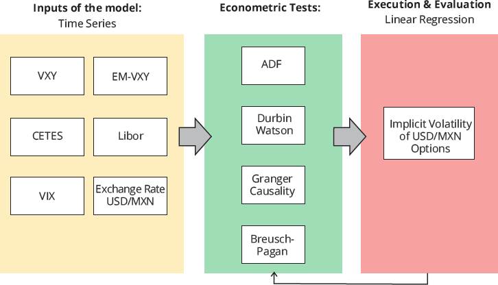
For the development of the implicit volatility model, a methodology is defined as shown in Figure 4, where we propose to test the above hypotheses. We submit the time series to econometric tests to validate that they are suitable for analysis and for exploring possible causalities toward the target variables, which is a prerequisite for applying the proposed model (see Figure 4).
Source: Prepared by the authors.
Figure 4 Diagram of the methodology for the implied volatility model of USD/MXN exchange rate options
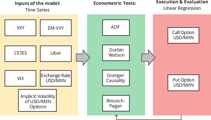
Additional variables, such as the CETES rate, the LIBOR rate, the VIX, and the USD/ MXN exchange rate are included in the list of inputs to complement the research with other variables of interest. Figure 5 shows the same methodology as the implicit volatility model. The difference is that for the call and put option price models, implicit volatility is part of the list of inputs (see Figure 5).
Source: Prepared by the authors.
Figure 5 Diagram of the methodology for the models of premiums of call and put options of the USD/MXN exchange rate
The criteria and considerations relating to each component of the proposed methodology will be detailed in the next pages.
b) Econometric tests
i) Augmented Dickey-Fuller (ADF)
One of the attributes that a time series must have to be applied in an econometric model is stationarity. A time series is stationary when it meets three conditions: its mean, variance, and autocorrelation must be constant through time. Informal methods exist to determine these attributes, such as the visualization of the time series graph. However, we can use formal methods, such as the ADF test, to obtain a high degree of certainty. The ADF test is an extended version of the Dickey-Fuller test in which additional lags are included in the dependent variables to eliminate autocorrelation problems (Mushtaq, 2011).
For the application of this test, the following hypothesis is proposed:
Null hypothesis: There is a unit root (it is not stationary).
Alternative hypothesis: There is no unit root (the time series is stationary).
Subsequently, the ADF test is applied, including the constant and trend factors, and considering a horizon of three previous values, as follows:
where:
y = variable to which the ADF stationarity test is being applied
δi = coefficient for the delta term of the variable of interest at time
α = constant coefficient
β = time trend coefficient
Finally, the ADF statistics of the time series are obtained and compared with the critical value of the ADF test with a significance level of 5% equivalent to −3.41 to determine whether or not they are stationary.
For this research, this test was selected to determine the stationarity of the time series and confirm that they can be subjected to analysis and used for modeling.
ii) Granger causality
The Granger causality test is based on testing whether or not a causal relationship exists between two variables. “Causality is expressed as a measure of using past values of X for a prediction of Y compared to not using past values of X.” (İskenderoglu & Akdag, 2020, p. 109). This test can be used to identify which of the variables used as the model inputs have a causal relationship with the variables to be modeled. The restricted and complete models are represented by the following two equations:
Restricted model:
Complete model:
where:
y = variable assumed to be caused by χ
x = variable that is assumed to cause γ
αi = regression coefficient for γ, i number of samples in the past
βj = regression coefficient for χ, j number of samples in the past
n = maximum number of passed values to include in the model
c1 = constant term of the restricted model
c2 = constant term of the complete model
The null hypothesis of the Granger causality test refers to the fact that the variable X does not have a causal relationship with the variable Y. The alternative hypothesis is that the variable X does have a causal relationship with Y. The F statistic of the test is calculated using the coefficients of determination of the two models and is compared with a critical F statistic for 95% confidence.
In the context of this research, for the models of implicit volatility, call option premiums, and put option premiums of the USD/MXN exchange rate, the causal relationship of up to 15 past values is explored between the input and the target variables. For those past values that result in a statistically significant causality with a reliability of 95%, the degree corresponding to said past value will be selected. The intermediate past values between the current and oldest past values that were shown to be causal to pass them on to the next phase of econometric tests regardless of whether they were statistically significant or not will also be selected.
iii) Durbin-Watson
The Durbin-Watson statistic is a measure used to detect the presence of autocorrelation in the residuals of a linear regression model. This measure is used to assess whether the residuals of a model are independent and uncorrelated (White, 1992). The Durbin-Watson statistic is represented by the following equation:
where:
DW = Durbin-Watson statistic
Once the equation is calculated, a critical value is determined, which varies depending on the size of the sample and the level of significance desired. This test can have three possible results: reject the null hypothesis, not reject it, or an inconclusive result. The result will depend on the area in which the Durbin-Watson statistic is located with respect to the critical values, as shown in Figure 6. The critical values used in this investigation were as follows: dL1 = 1.758, dU1 = 1,779, dL2 = 2,221, and dU2 = 2,242 (see Figure 6).

This test was selected for the investigation to confirm the existence of a serial correlation between the results of the Granger causality test, which will help reinforce the result and prevent it from being spurious. Those variables that have been selected after the Granger causality test but without a serial correlation after performing the Durbin-Watson test will be discarded.
iv) Linear regression (OLS)
The Granger causality test and a regression analysis enable the understanding of the effects of one index over another, as proposed by İskenderoglu and Akdag (2020) for the research of the causality of the VIX over the BIST-100 index. This research proposes to use the ordinary least squares (OLS) method to reveal the effects of the variables of interest and their past values whose selection comes from the results of the econometric tests previously mentioned.
The OLS regression is generated with the selected variables and the intercept for the implicit volatility models of the USD/MXN exchange rate options, including for the models of premiums in call and put options of these options. When any of the terms is not statistically significant, the least significant will be discarded. In addition, the intercept term and the regression will be generated again with the remaining terms. This process is repeated until only significant variables remain or, failing that, all variables have been discarded. In this case, the causality hypothesis will be rejected.
v) Breusch-Pagan
According to Breusch and Pagan, when the homoscedasticity requirements of a linear model are not met, the loss of efficiency of the OLS regression methods can cause misinterpretations and biases in the model results (Breusch & Pagan, 1979). Thus, the Breusch-Pagan heteroscedasticity test is included as part of the methodology. The final model resulting from the implementation of the OLS method will be used to make predictions on the objective time series with which it was developed. A new time series equivalent to the squared residual of each sample will be calculated.
A regression is carried out using the OLS method as independent variables used in the final model and using the previously calculated residual squares as the dependent variable. The regression equation for the squared residuals is as follows:
where:
δi = regression coefficient for the independent variable i of the final model
xi = independent variable i of the final model
c = constant term
The null hypothesis of the Breusch-Pagan test dictates that the model residuals have no heteroscedasticity. The alternate hypothesis dictates that heteroscedasticity exists in them. The chi2 statistic is calculated by multiplying the number of observations by the coefficient of determination of the regression of square residuals. With this statistic, a right-tailed chi2 test is performed with a confidence level of 95%. The result of which will provide a p-value that will help determine if the null hypothesis is rejected.
If heteroscedasticity is found in the model, then the relationships found between the independent and dependent variables are candidates to be explored in future research under various and highly complex autoregressive models or even using a broad past value horizon in the test of Granger causality. The reason is that heteroscedasticity would not allow the interpretation of the results obtained from the regression model with certainty. If homoscedasticity is found, then the model results can be interpreted with great certainty.
5. Empirical results
a) ADF
The application of the ADF test to each of the time series of daily returns shows that stationarity exists at least within a horizon of three previous values. This result means that transforming the time series is not necessary and that the methodology can be continued in its current condition.
b) Granger causality
The results of the Granger causality test for the implicit volatility model of the USD/MXN exchange rate options indicate that previous values of the variables EM-VXY, LIBOR, and VIX are causal. The 11th to 15th previous values of the EM-VXY were identified as causal. For the LIBOR rate, the 4th previous value and the 8th to 15th previous value were identified as causal. For the VIX, only the first previous value was identified. According to the proposed methodology, a range from the 1st to the 15th previous value is selected for the EM-VXY and LIBOR variables, whereas only the 1st previous value is selected for the VIX variable.
The Granger causality test applied in the context of the model of premiums in the price of call options of the USD/MXN exchange rate highlights the variables VXY, EM-VXY, implied volatility, and VIX as causal factors. Of the VXY, the 4th to 15th previous values were identified as causal. From the EM-VXY index, causality was identified from the 9th to 15th previous values. The causality implied that volatility values are the 5th, 6th, and 7th previous values. Finally, for the VIX, only the 3rd previous value turned out to be causal. As in the case of the implicit volatility model, these results lead to the selection of previous values for the variables VXY and EMVXY corresponding to a range from the 1st to the 15th previous value. From another aspect, a range from the 1st to the 7th previous value is selected for the implicit volatility variable, whereas a range from the 1st to the 3rd previous value is applied for the VIX variable.
Finally, in the case of the price premium model in put options of the USD/MXN exchange rate, significant causality is found in the implicit volatility, exchange rate, and VIX variables. In the case of implicit volatility, the first, second, and third previous values are identified as causal. For the exchange rate, causality is identified from the 1st to the 11th previous value. For the VIX, causality was only identified in the 1st previous value. The value ranges selected according to the methodology are from first to third for implicit volatility, from 1st to 11th for the exchange rate, and only the 1st previous value for the VIX.
c) Durbin-Watson
The results of the Durbin-Watson test for the implicit volatility model led to the discarding of the first previous value of the EM-VXY variable, whereas the rest of the variables selected after the Granger causality test were retained. For the model of premiums in put option prices for the USD/MXN exchange rate, all the variables identified after applying the Granger causality test were kept.
From another aspect, in the case of the model of premiums in call option prices, all the variables selected after performing the Granger causality test were discarded according to the results indicated in Annex 1. This result leads to the interpretation that the causalities found were spurious. Thus, the remaining steps of the methodology for this model will not be carried out (see Annex 1).
d) Linear regression (OLS)
Starting from the remaining variables after the application of the econometric tests, we proceed to implement a series of actions corresponding to the modeling using the OLS method. Table 3 shows the resulting variables for the implicit volatility model of the USD/MXN exchange rate options that were statistically significant. These variables correspond to lag 9 of the EM-VXY variable, lags 7 and 8 of the LIBOR variable, and lag 1 of the VIX variable. The coefficient of determination R2 of the model is 0.137 (see Table 3).
Table 3 Implied volatility model of USD/MXN exchange rate options
| Variable | Coef. | Standard error | t | p-Value | R2 | R2 adjusted |
| em_lag9 | −0.2281 | 0.074 | −3,093 | 0.002 | 0.137 | 0.122 |
| libor_lag7 | −0.1448 | 0.049 | −2,944 | 0.004 | ||
| libor_lag8 | 0.1678 | 0.049 | 3,393 | 0.001 | ||
| vix_lag1 | 0.0688 | 0.021 | 3,214 | 0.001 |
Source: Prepared by the authors.
The results obtained suggest that the implicit volatility of the USD/MXN exchange rate options can be modeled through Eq. (7).
where:
EMLag9 = value of the EM-VXY index 9 days prior to the forecast date.
LlB0RLag7 = LIBOR rate value 7 days prior to the prediction date.
LlB0RLag8 = LIBOR rate value 8 days prior to the prediction date.
VIXLagl = value of the VIX 1 day prior to the prediction date.
For the USD/MXN exchange rate put option price premium model, a list of variables survived the econometric tests. However, the results of the OLS method indicated that none of these variables was statistically significant for the modeling of the target variable. Notably, OLS regression is not carried out for the call option premium model for the USD/MXN exchange rate because all variables were discarded after the Durbin-Watson test.
e) Breusch-Pagan
Carrying out the Breusch-Pagan test for the implicit volatility model of the USD/ MXN exchange rate options shows that homoscedasticity exists in the residuals of the model with a reliability of 95%, as shown in Table 4. These results allow us to interpret the results of the proposed methodology, considering that there is a high level of certainty that the variance of the model has no undetected pattern or behavior that should be analyzed in depth (see Table 4).
6. Conclusions
After the application of the econometric tests, the modeling proposed to the time series indicates that a causal relationship exists between the EM-VXY and VIX indices and the LIBOR rate toward the implicit volatility of the USD/MXN exchange rate options. However, the VXY index is discarded as part of the model. Thus, implied volatility can be influenced by movements in emerging country currency-implied volatility indices and by the S&P500 stock options index and LIBOR rate.
The results of the coefficients indicate that a positive movement of 10,000 base points in the returns of the EM-VXY index nine days prior would inversely affect the next value of implied volatility for a value equal to −0.2281 or −22.81%.
Regarding the additional variables considered in the model, the effect of the same movement in the LIBOR rate seven days prior would be −0.1448 or −14.48%, whereas that of a movement of this rate eight days prior would be 0.1678. Therefore, this case would cause an increase of 16.78%. Finally, the VIX a day prior would cause a 0.0688 or 6.88% increase in implied volatility for every 10,000 base points.
Meanwhile, the variables selected for the model of the premiums in the call and put prices of the USD/MXN exchange rate options did not pass the stress tests or the significance criteria during the modeling. Therefore, the VXY and EM-VXY indices do not impact the prices of said premiums in the case of the contracts studied.
In terms of this research’s objective, the VXY and EM-VXY indices cannot predict future changes in implied volatility. Therefore, using them as input or output in investment strategies and risk hedging is not possible. Despite the aims they were designed for, these instruments fail to effectively capture the behavior of exchange rate markets through the implicit volatility of the currency options that comprise them. One possibility is that the markets’ reaction to real volatility is not consistent over time. Therefore, the implied volatilities that make up these indices are not of much use. Moreover, additional factors may influence emerging markets such as Mexico in a way that these instruments fail to capture.
The proposed methodology should be extended to study other currency pairs and exchange rates, using different combinations of rates for the calculation of the strike forward and the selection of contracts. Moreover, future studies should explore additional modeling techniques and even artificial intelligence algorithms that could greatly capture the complexity of the markets while providing information on the influence of independent variables in the predictive process.
Further study of this topic is of great relevance owing to the significant impact of volatility in financial markets in terms of investment, coverage, and risk reduction strategies.

