


 nueva página del texto (beta)
 Inglés (pdf)
 Artículo en XML
 Referencias del artículo
 Enviar artículo por email
 Citado por SciELO
  Similares en
SciELO
Similares en
SciELO 
 Permalink
1. Introduction
Financial markets participants use early indicators to assess changes in the business cycle, which can be instrumental for successful investment choices such as to reallocate among asset classes or to hedge positions. In this logic, Gajewski (2014) shows that Markit PMI Composite (Purchasing Manager’s Index) produces the strongest statistical relationship with quarterly GDP growth rates when compared with a group of popular business cycle indicators in several European countries. Moreover, other studies explore the use of early indicators of business cycle to build strategies that show potential for fund managers and risk professionals interested in active investment strategies. For instance, Peláez (2015) shows that using the probability of recession in-advance (for which ISM is used) and a group of naïve investment rules in which there is a switch between holding a S&P 500 index fund and T-bills and returning to the index after a predetermined number of months, an investor could outperform a strategy of buy and hold the S&P 500 in final wealth in the period 1970-2014. There have been other papers study active strategies using different business cycle leading indicators, such as OECD’s CLI (Organization for Economic Cooperation and Development, Composite Leading Indicator). As mentioned by Dzikevičius and Vetrov (2012b) it is sometimes stated that the current state of the economy influences the determination and movement of stock prices. To contrast the above between March 1955 to May 2011, they used the CLI indicator to determine the economic cycle of the set of stocks comprised within an investment portfolio. They found that this indicator could anticipate the movements of the economic cycle, and thus modify the weightings of the stocks and achieve better return/risk efficiency in the portfolio. In another study these authors (Dzikevičius & Vetrov, 2012a) included other financial assets to verify that the OECD indicator could provide information on return expectations. They found that asset classes behave in a different way along the OECD business cycle, showing that the CLI can provide significant information on financial market expectations. In a later work, Dzikevičius & Vetrov (2013) use the CLI to define business cycle stages and optimize portfolios with different restrictions in each phase of the economic cycle, finding that cyclical asset allocation outperforms passive strategies. In other instance, Celebi & Hönig (2019) identify a relationship between CLI movements, and stock yields in subsequent periods, also showing that in economic crisis, these indicators had a significant impact on returns compared to pre-crisis and post-crisis periods.
This paper proposes a naïve investment strategy, like others in the relevant literature, however, such strategy is based on an innovative hypothesis: the bias associated to managers sentiment present in the BCI. That is, when managers are surveyed about their opinion, they give a biased appraisal, when compared with a data-based indicator, such as the CLI. This bias produces a gap between both indicators, and this is used to determine the portfolio composition between a stock index and a short-term government bond.
The work is organized in four sections besides this introduction. The second part briefly elaborates about the two indicators used and the source of the bias, followed by the investment strategy proposed in the paper. In the fourth section, main results are presented and analyzed and in the final section, conclusions are presented.
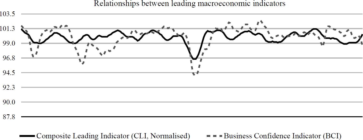
There are several methodologies to build such indicators, however, they can be classified by the source of information used to build them. Under these assumptions, there are indicators based on sentiment surveys (e.g. Markit’s PMI, Conference Board’s CCI, OECD’s BCI, etc.), and, on the other hand, there are composite indicators based on data series (e.g. Conference Board’s LEI, OECD’s CLI, etc.). The main difference between the two types of indicators is that the ones that use surveys as input contain elements of judgement about the future of business climate, while the economic data used as the base for composite indicators does not. For instance, OECD’s Composite Leading Indicator (CLI) purpose is to signal of the near future change in the business cycle and for its construction the OECD uses economic time-series data that exhibit a leading behavior regarding the GDP (OECD, 2019a). This differs from OECD’s Business Confidence Index (BCI), which is based on opinion surveys in the industry sector (OECD, 2019b). This difference may be crucial since sentiment surveys may be subject to several bias instances. Although this issue has not been extensively studied on economic sentiment surveys, it has been researched in other types of surveys and it can be conjectured that some of these biases are also present in sentiment surveys.
The interpretation of the spread between CLI and BCI and its use for an investment strategy is not present in the relevant literature regarding leading indicators, and it represents the main contribution of this paper. To illustrate the strategy and its results the Mexican financial market is used without loss of generality. All the procedures can be easily replied or adapted to any other financial market. Results indicate that using the interpretation of the spread and the proposed strategy increases the probability of getting a higher yield and decreases the probability of negative yields when compared with the buy and hold the average stock market portfolio.
There are other studies that seek to improve the productive power of CLI. For example, Wong et al. (2014) identify the business cycle through dynamic factors which better identifies the business climate and economic shocks in Malaya, compared to the CLI. Tkacova et al. (2017) after analyzing 140 indicators and the application of data processing methods create an indicator for Germany which outperforms the OECD CLI. Vraná (2018) develops an indicator that differs from the CLI indicator developed by the OECD, whose composition depends solely on national data. This indicator takes into account the strong relationship that some countries of the European Union have.
2. Methods, techniques, and instruments
Portfolio optimization is performed in each of the four stages of the economic cycle. Unlike in this document, the optimization is throughout the period, through monthly decisions of the movement of a percentage of capital between investments in variable income (Mexican stock exchange index, IPC) and fixed income (Mexican treasury bonds, CETES).
The OECD’s CLI indicator is based on the «cycle growth» approach, in which business cycles and tipping points are measured and identified as deviations from the series trend. Gross Domestic Product (GDP) is the variable used as a reference for the identification of turning points in the growth cycle in all countries (OECD, 2019a). This way, the CLI can be used for the construction of a decision rule of the weights of an investment portfolio.
In Mexico, the construction of the CLI uses various variables related to employment in the manufacturing sector, production, 10-year bond interest rates, capture costs and the real exchange rate (OECD, 2019b). This allows the CLI to capture highly sensitive information for the Mexican economy, such as that related to the external sector, which is the most dynamic component of aggregate demand (Palley, 2012). That is to say, it captures information with high influence in the determination of the GDP, and in that sense, it allows to anticipate instead in the tendency of the latter.
The variable to optimize is the percentage of capital movement between fixed income (CETES) and variable income (IPC) during each month, taking into account transaction costs (see Table 1).
Table 1 Simulation results for optimization period: 1998-2018.
| Rolling windows returns | |||||
| Asset allocation (% of capital) | Portfolio anual geometric yield | IPC annual geometric yield | Average weight of investment in IPC (%) | Average weight of investment in risk-free (%) | |
| 10 % | 13.7 % | 11.1 % | 41.9 % | 58.1 % | |
| Optimal portfolio | 25 % | 15.4 % | 11.1 % | 39.8 % | 60.2 % |
| 50 % | 15.2 % | 11.1 % | 39.6 % | 60.4 % | |
| 75 % | 14.9 % | 11.1 % | 39.7 % | 60.3 % | |
| 100 % | 14.7 % | 11.1 % | 39.8 % | 60.2 % | |
| With leverage (200 %) | 25 % | 25.6 % | 11.1 % | 39.8 % | 60.2 % |
Note: Transaction costs of 0.25 % + tax for each purchase or sale of financial instruments are considered.
CETES was taken as the risk-free rate. IPC is Mexico’s stock exchange index.
Source: Own construction.
Not every month (end of month) there are capital movements, for example if the investment rule calls for a 25 % movement in fixed income and currently the fixed income has 100 % of the capital, this movement is not made. Likewise, if the rule asks for 30 % in fixed income and currently the fixed income has 90 % of the capital, only 10 % of the movement of the capital is carried out, since the investment heuristic does not allow investments higher than 100 %. Therefore, let 𝜃 denotes the optimal change in capital invested to achieve the largest ending balance on the investment horizon.
Where the portfolio return is 𝑟𝑝 = 𝑤𝑡 × 𝑟𝐼𝑃𝐶 + (1 − 𝑤𝑡) × 𝑟𝐶𝐸𝑇𝐸𝑆
Monthly data from the CLI (normalized, OECD), BCI (Business Confidence Indicator, OECD), monthly closing prices of the IPC (Infosel database) and the 28-day CETES interest rate (Banxico database) are used for the period from January 1998 to May 2021. Where the decision rule is based on the differential between the CLI and the BCI (see Figure 1). It takes into account a delay of two months for the publication and adjustments that may have the OECD variables.
3. Results and discussion
Like Dzikevičius and Vetrov (2012a), it seeks to take advantage of the movements of the economic cycle, to increase the performance of a portfolio and contrary to what was found by Han, Li & Yin (2018), where the economic cycles studied through the CLI do not fully reflect the real conditions of the stock markets.
The dynamic asset allocation strategy being developed is really simple, but far exceeds the market (measured by the country index, IPC). Figure 2 shows the analysis of the strategy over time (portfolio), clearly, the strategy improves the value of the portfolio in the period analyzed was higher than the market. With an annual geometric rate of 15.4 %, against 11.1 % from the market, which gives us a differential of 4.3 %. This was achieved with an average investment of 39.8 % in variable income (IPC) and 60.2 % in the risk-free rate (CETES). The dynamic strategy is reviewed every month, and if necessary, the portfolio is balanced up to 25 % of the capital. See in Table 1, the simulation with other percentages of dynamic capital allocation (asset allocation).
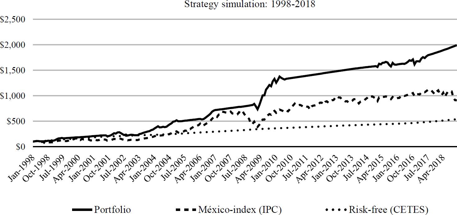
Source: Own construction.
Figure 2 Portfolio vs México-index (IPC) into the optimization period: 1998-2018. Dynamic investment strategy (Portfolio) outperforms in return and with less pronounced negative returns.
It would be a mistake only to evaluate the analysis of the strategy with Figure 2, it is possible to have different investment horizons during the period analyzed. Figure 3 shows four different investment horizons (12, 6, 3 and 1 month), rolling window was used to include the maximum number of investments within the period. Where the frequency distribution of yields for the developed strategy presents a greater kurtosis and a lesser bias towards negative yields.
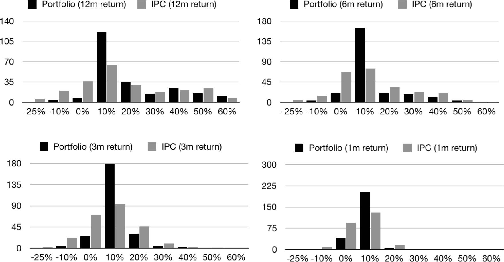
Source: Own construction.
Figure 3 Histograms at different horizons of investments: rolling windows returns 1998-2018. For the four investment horizons, the IPC had a higher frequency at the extremes into the optimization period.
Table 2 compares portfolios that use the strategy to one and ten years, also rolling windows is used to take maximum advantage of the observations within the period studied. Using a dynamic balance in the asset allocation of 25 %, a yield higher than the stock exchange index is obtained in 47.5 % and 57.6 % of the observations respectively for both portfolios. And in terms of risk, there is a 5 % of negative returns to a year in the portfolio against 25.8 % in the IPC. The portfolio in the analyzed period has a maximum drawdown of -23.4 % against -44.5 % in the IPC. In case of having the possibility of leverage (2 times) 100 % of the observations are exceeded in 10-year returns to the IPC, having a maximum drawdown lower than the IPC (-42.8 and -44.5 % respectively).
Table 2 Portfolio analysis at 1 and 10 years, 1998-2018.
| Rolling windows returns | |||||||
| Asset allocation (% of capital) | Probability of beating IPC in 1year investments | Probability of beating IPC in 10year investments | (%) of Portfolios with negative annual yields | (%) of IPC portfolios with negative annual yields | Portfolio Maximum Drawdown | IPC máximum Drawdown | |
| 10 % | 42.9 % | 42.4 % | 5.8 % | 25.8 % | -24.3 % | -44.5 % | |
| Optimal portfolio | 25 % | 47.5 % | 57.6 % | 5.0 % | 25.8 % | -23.4 % | -44.5 % |
| 50 % | 45.0 % | 44.7 % | 7.1 % | 25.8 % | -23.4 % | -44.5 % | |
| 75 % | 41.7 % | 41.7 % | 7.5 % | 25.8 % | -23.4 % | -44.5 % | |
| 100 % | 40.8 % | 37.1 % | 7.9 % | 25.8 % | -23.4 % | -44.5 % | |
| With leverage (200 %) | 25 % | 67.5 % | 100.0 % | 8.3 % | 25.8 % | -42.8 % | -44.5 % |
Note: The optimal portfolio implies movements of 25 % of the capital during each month, other simulations are shown to compare results. If leverage is available, during the period analyzed, the portfolio exceeds the IPC by 100 % of the observations at 10-year investment horizon.
Source: Own construction.
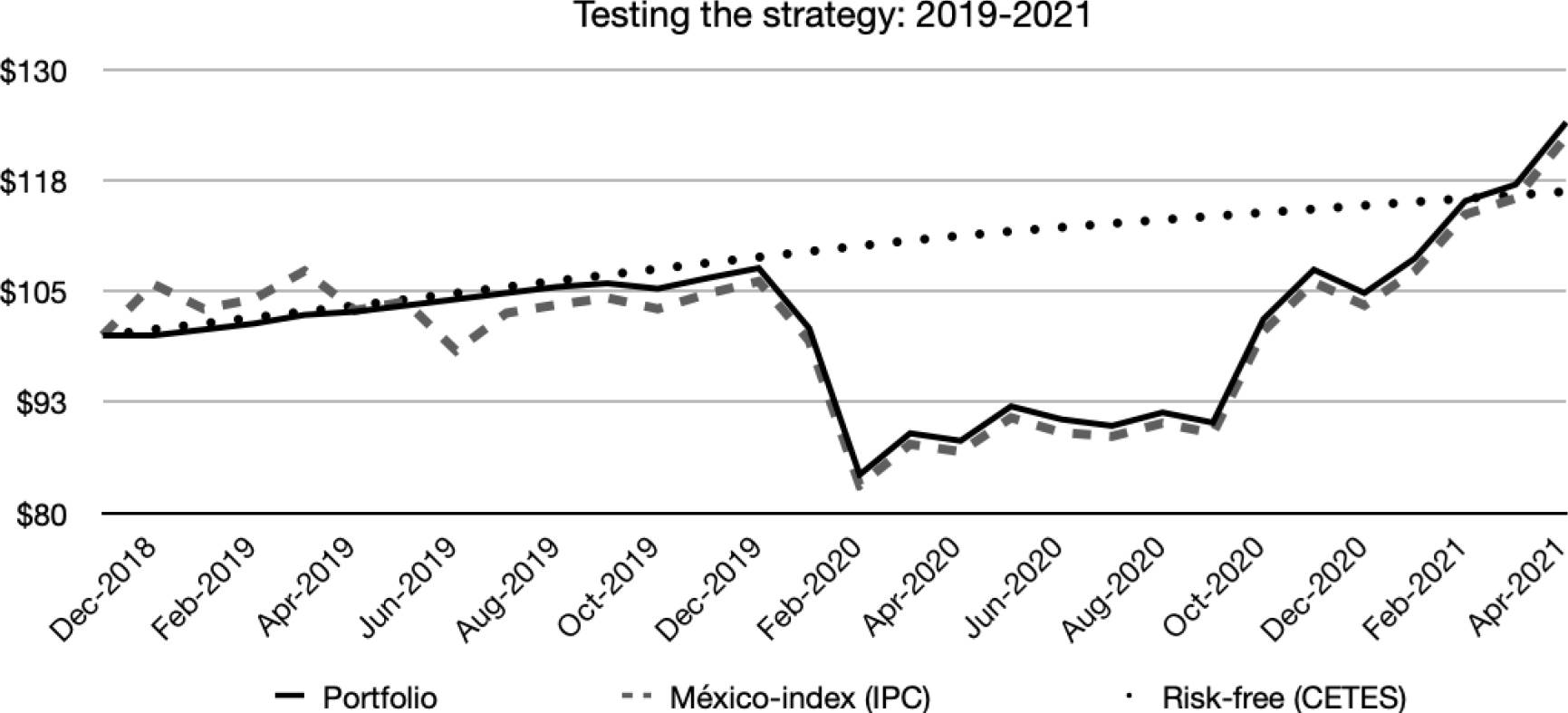
Until now the portfolio is optimized in the period 1998-2018. Figure 4 contrasts the strategy outside the optimization period, between January 2019 and May 2021. At the beginning of the period until November 2019 the portfolio remains invested in CETES, giving the portfolio a more stable growth compared to the IPC. Subsequently, it is invested in the IPC and the strategy does not manage to anticipate the fall of the IPC. But from July 2019 to May 2021 the portfolio maintains a higher balance than the IPC and ends with the highest balance.
4. Conclusions
The hypothesis where the investor seeks to maximize his utility through undiversified portfolios must be rejected (Markowitz, 1952). The investor seeks diversified portfolios that can take into account the imperfections of the market, be a guide for the investor's behavior. These imperfections can be caused by the economic cycle. Cervantes et al. (2016) conclude that there is a relationship between the economic cycle and short-term investment strategies. A dynamic model is presented that links the predictability of profitability but based on a single systematic factor and in a simpler way, considering the differences between sentiment and data. The investment strategy balances capital each month taking advantage of the economic cycle forecast through the CLI. It dynamically changes up to 25 % of capital, in investments in the Mexican stock exchange index and in CETES. In the optimization period 1998-2018, a differential of 4.3 % (geometric mean differential) compared to the market was achieved. During the contrast of the strategy between 2019-2021 the differences with the IPC were not significant, but higher most of the time.
There are developments of this type of indicators in the literature (Tkacova et al., 2017; Wong et al., 2014), which can improve the one proposed by the OECD. Although the results are statistically positive and higher than the market index (IPC). It is necessary long investment periods in time to show a high differential in capital. It is suggested for future lines of research to develop a leading indicator for the market in question.

