


 nueva página del texto (beta)
 Inglés (pdf)
 Artículo en XML
 Referencias del artículo
 Enviar artículo por email
 Citado por SciELO
  Similares en
SciELO
Similares en
SciELO 
 Permalink
1. Introduction
Nowadays supply chains require operational strategies to remain competitive in the market. Competitiveness is not only based on having low costs, but companies must have good quality products, manufacture them quickly and meet delivery times, as well as be flexible and innovative (Coello & Tobar, 2018). On the other hand, it is known that supply chain consists of joint activities between suppliers and connected customers that allow to respond to the demand; It is sought that the execution of the activities be coordinated with the flow of the whole chain and, in this way, respond in a timely manner to the customer. Therefore, supply chain management allows to have a strategic view on the management of inputs and flow within the internal and external processes of the company, with the aim of making each link in the chain more efficient (Aldana-Bernal & Bernal-Torres, 2018).
Within this context, transport and distribution management is established as one of the macroprocesses of comprehensive logistics management, it involves all activities directly or indirectly related to the need of placing the products in the corresponding destination locations, according to the level of service, security and costs (Mora, 2016). Logistics operations influence this dimension directly and companies have chosen to implement mathematical models to make safer decisions that optimize resources (Gil, 2018).
Mathematical models are tools that allow to optimize operations that present different options for making decisions, where the model helps to determine the best way to use resources, based on the most representative variables and parameters of the system (García-Cáceres et al., 2018).
Therefore, these models are currently quite effective in the use of transport resources, because they allow the reduction of travel time, distances covered by the vehicles and the reduction of costs, which ultimately improve customer service. All this is obtained by processing the information of the production, distribution and consumer centers (Mora, 2016). As a result, models have been developed for various distribution and transport systems that allow special considerations, such as variety of products and vehicle capacity, to be taken into account. Below the transshipment problem and the Travelling Salesman Problem (TSP) are presented since they have been frequently used in this field.
Transshipment problem. In a system where goods are shipped between supply points to demand points and at the same time, there are intermediate points that connect both classes, it is necessary to define which paths require less resources (time, distance, cost) to meet a demand (Winston, 2004). The transshipment problem has different variants that allow it to be applied in other systems with more specific requirements, such as the capacitated transshipment and open transshipment models. The Capacitated Transshipment Model (CTP) takes into account that for each arc that joins two points it has a maximum resource flow capacity; on the other hand, the Open Transfer Model (OTM) has the option that supply points can receive resources from another point, as well as with the demanding points, where they have the ability to supply resources to other points.
Travelling Salesman Problem (TSP). In a system that has all the points connected to each other, the shortest distance that joins all points is to be found. Although initially used for distances between cities, this problem has applications in other areas, such as in production systems or biological structures (Melo, 2019).
In this regard, this work addresses a problem of the distribution of products in the city of Bogotá, in order to meet the weekly demand for 22 consumer centers of 6 references of soft drinks, through 3 production centers and the availability of 3 distribution centers. Because of transportation costs are relevant to the company profits, it is necessary to establish how to distribute the products with the least time, displacement and therefore cost. For this reason, this study develops a mathematical model based on Mixed Integer Programming (MIP) to establish the weekly vehicle travel, taking into account the capabilities of production centers, vehicle capacity (by weight and volume) and demand in each consumer center. On the other hand, the company requires determining the performance of the logistics network by implementing electric vehicles, in order to improve environmental indicators, but without sacrificing the levels of vehicle utilization, time and distance required. (Di Nucci, 2013)
This article is organized as follows: Section 2 presents the literature review, the basis for the development of the study. Section 3 presents the methodology used in the investigation. Section 4 presents the context of the company subject of the applied model. Section 5 presents the model development process that indicates a solution alternative to the problem stated. Finally, Section 6 presents the results of the models used and the conclusions in Section 7.
2. Literature review
The articles and publications cited in this section are related to route optimization, transshipment models, multi-product models and vehicle capacity management.
A Linear Programming (LP) and Mixed Integer Programming (MIP) model to minimize fixed costs and variable transportation costs with better operating levels is proposed in (Marmolejo et al., 2015) and in (Herrera et al., 2019) using GAMS Software. The first study seeks to establish a network of arcs, which allows the flow of products to meet the demand of distribution centers and the possibility of maintaining a high level of customer service. The second one performs the design of the mathematical model of the transport system from the third-order cybernetics structure, integrating the delivery of several products from plants to customers with transshipment centers.
Another research relates to the formulation of optimal routes, it is applied to the integral urban transport system area in Bucaramanga, Santander. They (Marín & Melendez, 2017) presented the design of a restricted transport network, from the Vehicle Routing Problem with Time Windows (VRPTW) approach to decrease distances and travel times. The model established capacity and time constraints on travel and demand by sector.
The multiplicity of products is emphasized in (Zhang & Chen, 2014) and in (Imariouh et al., 2017). The latter study presented a distribution model for a water bottling company, where there were several sizes of bottled water to be sent from a supplier to a set of Morocco's regional warehouses and wholesalers. The objective of this MIP model is to create a plan that will adjust distribution and inventory management decisions to achieve reduced operational costs. The situation presented is an Inventory Routing Problem (IRP), where pallets were set as shipping units, making proportionality ratios between products to facilitate the management of capacities. The former (Zhang & Chen, 2014) addressed a vehicle programming problem, based on the logistics of the cold chain for the delivery of variety of frozen foods. The Vehicle Routing problem optimization model (VRP) seeks to find the minimum delivery cost, which is made up of the costs of the following areas: transportation, refrigeration, cargo damage of frozen products and customer penalty. There are combinations of limitations of time frames and load weight plus considering the unit volume of the different frozen foods to establish vehicle volume capacity restrictions.
Likewise, the VRP covered in (Botero Gómez, 2018) is proposed as a logistic model for perishable products under the "Last Mile" approach using GAMS Software to identify distribution routes seeking to maximize profits and decrease transport times taking into account factors such as number of vehicles, types of vehicles with their respective capacities, demands and transportation costs. In turn, a heuristic comparison of this same problem is made using GAMS software (Fajardo et al., 2016), proposing solution methods with two approaches; the first one, an application of the Clarke and Wright savings algorithm where the number of vehicles is not fixed, a decision variable that seeks to reduce the number of vehicles to use and reduce the distances traveled. The second one is the implementation of the TSP optimization model, obtaining as a result the method with optimal values in distances, costs and travel times for the collection of used lubricating oils in the city of Pereira, Colombia.
With regard to transshipment models, which are a variation of the conventional transport problem, a recent work (Tawanda, 2017) developed a new approach to solve the transshipment problem, where transport problem algorithms and methods are applied for transforming and solving a transshipment model. This method consists of merging the source nodes with the transshipment nodes, using all possible join connections. On the other hand, recent publications (Agadaga & Akpan, 2019) introduces a soda transport model of the bottling company Seven-Up as a LP transshipment model with the aim of minimizing the transportation cost of 10,000 bottle crates from its location in Benin, through transfer points to the Sa-pele-Warri region. This model has two types of nodes: (i) sources or suppliers (production plants) and (ii) sinks or demanders (retails outlets), likewise, a homogeneous set of products are handled, so demands are not differentiated; in addition to this, demand for the 11 outlets located in Nigeria's Delta state is handled in crates delivered weekly. A design of a hybrid model is proposed in (Ochoa & Fonseca, 2018) to determine the route based on the shortest distance for the logistics distribution operation for Small and Medium Enterprises (SMEs) of dry cargo in Bogota; its first stage considers the transshipment operation based on a combined load allocation model as a classic transshipment model and in its second one the specific routing of that operation is proposed.
In general, when solving transport and distribution problems, complications arise from the need to identify variables that influence the system, which increase the complexity of the problem, such as system limitations and restrictions. That is the case of the capacity of vehicles which is considered as one of the factors for route assignment (Lahrichi et al., 2015) and (Benito, 2015). That research proposes an approach based on a scenario analysis to determine the best milk pick-up routes from farms to processing plants. This problem is known as the Dairy Transportation Problem (DTP), that deals with the efficient management of milk transport. In this particular case, the warehouses hold a different number of vehicles with different capacities, where a utilization limit parameter is used to limit capacity. From another viewpoint (Lmariouh et al., 2017), the goal is to find routes that represent the minimum cost of delivery for a fleet of vehicles with homogeneous capacity.
From this literature review, it can be concluded that in the development of VRPs some studies cover the topic of heuristics and variations such as transshipment problems. In addition, LP and MIP models and solvers are largely used, noting the preference for the use of GAMS Software. Therefore, this research study aims to cover a transshipment problem by exploring some variations to contribute methodologically and to apply it to a case study.
3. Methodology
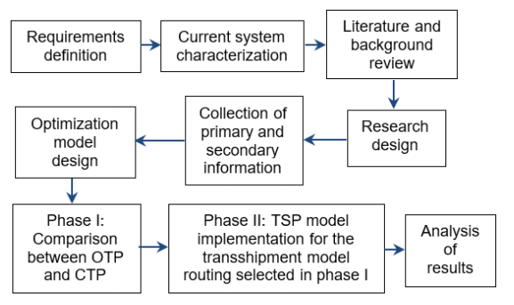
Figure 1 presents the process used for the development of the study, which begins with the definition of the needs of the soda company to optimize the planning of the weekly distribution up to the analysis of the results.
4. Application context
The application area of this study covered the logistics of distribution operation of a Colombian company producing sugary drinks, fruit drinks and water located in the city of Bogotá. This company starts up its production process with the production of beverages at the production centers, and then they are optionally taken to the distribution centers to be stored and sold at different retailer’s outlets. The company initiates a process of planning and reviewing its distribution strategy, thinking about being environmentally friendly. In this context, the company adopted a new strategy deciding to implement the use of zero-emission trucks to reduce the carbon footprint. Therefore, the analysis of the implementation of an electric vehicle inclusion campaign for the company's logistics distribution operation is carried out.
4.1. Characterization of the problem
The general outline of the problem is shown in Figure 2.
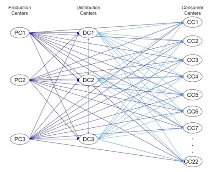
As shown in Figure 2, the company must distribute its products from three Production Centers (PCs) to 22 Consumer Centers (CCs) located in Bogota, whether or not using three Distribution Centers (DCs). In response to this demand, the company has vehicles with higher capacity at the production centers and vehicles with lower capacity at the distribution centers for the delivery of the products, being those of lower capacity vehicles of the electric type due to the company's consideration in implementing environmentally friendly technologies. On the other hand, two Production Centers (PCs) manufacture sodas and juices, while the third one produces bottled water.
The study handled the products in packaging units called "paca" (a colloquialism for pack), characterized by its weight and volume measurements that were added to the model as capacity constraints. There are two types of vehicles defined in the model. The first is the electric type vehicle that has a low operating expense, although it has a low capacity. The second one is a truck type that has higher capacity but has high operation costs. Table 1 illustrates the characteristics of both vehicles.
Table 1 Vehicle features.
| Electric-type vehicle | Truck |
|---|---|
| Brand: Renault Kangoo Z-E | Brand: Hino FC9J Truck |
| Capacity: 650 kilograms or 3,000 liters | Capacity: 6,500 kilograms or 7,800 liters |
| Total cost per km: USD: 0.095 | Total cost per km: US 0.75 |
This works develops an application with a technical approach based on historical data collected from secondary sources of information and direct observation. The most influential variables in the company distribution operation, their obtaining source and the tool used are listed in Table 2.
Table 2 Source and information-obtaining tool.
| Data type | Obtaining source and means | Tool used |
|---|---|---|
| Demand Supply | Primary and Secondary Information. | Observation Websites |
| - Product Information (Volume and Weight) | Primary information | Observation Measurement |
| - Fixed Costs and Variable Transportation Costs | Secondary information. Companies in the sector | Annual reports of transport prices in the city of Bogota Vehicle Business Websites |
| Distances between production centers and customers. Distances between production centers and distribution centers. Distances between distribution centers and customers. | Secondary information Web application | Google Maps |
| - Vehicle routes for the distributing goods. | Secondary information Web application | Google Maps |
| - Vehicle data | Secondary information | Vehicle Business Websites Car performance reports. |
| - Allocation of cargo production centers, distribution centers and customers. | Optimization Model. Computational application | Software GAMS LP |
Certain aspects such as the market exchange rate (MER - Colombian Pesos per Dollar) were taken into account for the study's development, therefore transportation costs were estimated in US dollars, using the average exchange rate obtained between October 2019 and November 2020, i.e., $1 USD = $3,391 COP. The model considers the capacity constraints of volume and weight in the two types of vehicles; the volume values measured in liters and the weight measured in kilograms of each pack or bale. On the other hand, the model in phase I, does not take into account time restrictions, the result of the model is oriented to indicate the number of trips to be made weekly to each distribution center and consumer centers defining the type and quantity of products to be transported by each type of vehicle. Phase II addresses routing, which takes into account the best outcome of phase I, to select trips that have a low level of use of vehicle capabilities in order to make trips that meet both the demand of consumer centers and have a higher level of capacity utilization.
5. Model approach
The model was designed based on vehicle characteristics and the number of supply and demand nodes. Therefore, the routing allocation is determined by both fixed and variable costs, taking into account that the fleet of vehicles varies depending on the place of departure, that is, the trucks will be used in the PCs and the electric type vehicles will be used on the DCs. The model was design in two phases with the objective of finding the fewest routes as possible. The first phase allocates trips that meet the demand for products from all CCs at the lowest cost. Based on that, trips with low vehicle capacity utilization are used for the second phase in order to perform a single journey or delivery routing between PCs and DCs with the respective assignments determined in phase I. The models used in both phases are based on mixed integer programming.
Phase I: Trips assignment:
At this stage, a Capacitated Transshipment Model (CTM) and an Open Transshipment Model (OTM) were made, with the purpose of compare them and then choose the best results, i.e. the model with the lowest number of trips and the lowest total cost. Tables 3 and 4 define the variables and parameters used in both models the CTM and OTM respectively.
Table 3 CTM and OTM variables.
| Notation | Description |
|---|---|
| Xhij | Number of product units h to be shipped from output node i to arrival node j in one week. |
| Yij | Number of trips required from the output node i to the arrival node j in one week. |
| Zij | Weight flow to be sent from output node i to arrival node j. |
| Wij | Volume flow to be sent from output node i to arrival node j. |
| Kij | Number of trips required determined by the unrounded weight from the output node i to the arrival node j. |
| Jij | Number of trips required determined by the unrounded volume from the output node i to the arrival node j. |
| Mij | Residual variable of vehicles determined by weight from output node i to arrival node j. |
| Nij | Residual variable of vehicles determined by volume from output node i to arrival node j. |
Table 4 CTM and OTM parameters.
| Notation | Description |
|---|---|
| CFij | Fixed cost of travel from output node i to arrival node j. |
| Cuhij | Unit cost of product h from output node i to arrival node j. |
| Puh | Unit weight of product h. |
| Vuh | Unit volume of product h. |
| Fpij | Conversion factors for the weight capacity of the trip from the output node i to the arrival node j. |
| Fvij | Conversion factor for the volume capacity of the trip from the output node i to the arrival node j. |
| Lhj | Product demand/supply h by node type j. Node j is demanding if Lhj < 0; node j is transshipment center if Lhj x 0; node j is source if Lhj > 0 |
| Vmj | Maximum volume capacity per node type j. |
| Lp | Proportion of minimum boarding capacity determined by weight |
On the other hand, the particular structure of the CTM is shown below:
Subscripts
h: Product type. ∀ h = 1, 2, ..., 6
i: Output node ∀ i = 1, 2, ..., 28
j: Target node ∀ j = 1, 2, ..., 28
Subject to
Constraints are defined as follows: (2) allows the balance value of each product h for each type of node j, that is, if the node is a source (Lhj > 0), transshipment center (Lhj x 0) or demander (Lhj< 0). It is important to note that the supply and demand of the whole system must be the same. Equations (3) and (4) determine the weight and volume flow for each trip between node i and node j, respectively. The number of trips required for each route between node i and node j has defined a weight flow, determined in constraint (5), the volume flow of the required trips determined in the constraint (6) for each trip between node i and node j was determined as well. It should be noted that the values taken by Z and W are different for each route between node i and node j. Because of Zij and Wij represent trips with decimal fraction, Equations (7) and (8) allow you to obtain the number of trips required, where Mij and Nij absorb the difference to complete the integer number. Equation (9) allows us to set a maximum percentage of unused capacity of the vehicle (Lp) to send the last trip of the route between node i and node j. The restriction is determined by the vehicle's load capacity. Finally, Equations (10) and (11) define the type of variable, where the first equations have the non-negativity property, and the second ones are integer type variables.
Otherwise, the OTM has a difference in the restriction (2) with respect to the CTM, because the structure of the model determines supply and demand under different constraints, so it is necessary to create two new parameters set as follows: Aih: supply of node i of product h and Bhj: demand of product h to node j, and replace Equation (2) with the following set of restrictions:
The constraint (12) defines the amount of product h offered by node i, so these nodes behave as sources, while the constraint (13) represents the demand for product h at node j, so these nodes behave like sinks. Additionally, restrictions (14) and (15) were added to represents the source nodes as transshipment centers and sink nodes as transshipment centers, respectively. These restrictions only differ with constraints (12) and (13) in the way the ATih and BThj parameters are defined, because there must be a balance at a node between incoming and outcoming loads. Therefore, to get the balance property at the nodes as transshipment centers, the parameters are defined as follows:
Equation (16) defines that for a transshipment center node i that offers an amount At of product h, it is necessary to add the total system supply (adding the quantity offered by the same node). Similarly, for a transshipment center node j that demands a Bt amount of product h, it is necessary to add the total supply of the system. This must be done for all nodes that behave as a transshipment centers, so that they do not supply or demand products.
It should be noted that both models allow nodes as transshipment centers to supply and demand products; in the OTM they differ by the use of Equations (16) and (17), while in the CTM it is made by means of the parameter Lhj.
Phase II: Trips routing with low vehicle capacity utilization via TSP model
At this stage, the best solution was chosen among the phase I models determined by the shortest time, distance traveled and cost. From this, routes are carried out on assignments that have a low utilization of the vehicle's capacity to reduce the number of trips and obtain lower operating costs. Additionally, implementing the routing system is expected to improve capacity, distance, time, and cost indicators. Therefore, this section established the routes as follows:
1. Select an i node that allows inputs delivering, that is, a PC or DC.
2. Determine the minimum proportion of weight capacity usage (P) expected to be carried on each trip, for example, if P = 0.5 all trips are expected to exceed 50% in the weight capacity usage.
3.From the nodes assigned to node i on phase I, select trips that have lower capacity usage than expected, that is, if the variable Mij < P the trip Yij makes part of the route of node i.
4.Determine the maximum number of nodes that make part of the route for node i. For this, it is necessary to take into account the capacity of the vehicle to be used in the routing and the accumulated weight of the trips that were selected in step 3.
5.Determine the shortest path using the TSP model.
6. Repeat step 1 until all sources nodes are evaluated.
The TSP model mentioned in step 5 determines the shortest distance by going through all points only once and returning to the destination. For this, Yij is defined as a binary variable that activates the path from node i to node j when it is 1 or disable it when it is 0, and Ui defined as the stage at which node i is visited. On the other hand, the parameter Cij is defined to determine the cost of going from node i to node j, defining the structure of the TSP model as follows:
Subject to
6. Results
This section in the first instance presents the comparison of the results obtained by the CBC Algorithm, in the mathematical modeling tool GAMS, allowing the choice of assignments given by the CTM or OTM, described in phase I. Subsequently, the area covered and routing for the selected model will be displayed and finally, the improvements obtained when implementing the proposed system are exposed.
Table 5 shows a comparison of the indicators obtained for the two established models. It is noted that the OTM has a reduction in the time and travelled distance indicators of 2.6% and 14.67% respectively compared to the CTM, although it was 5% by weight and 4% in volume above it from the perspective of vehicle utilization. On the other hand, the total costs of the logistics distribution operation are very similar in the two models, being the OTM lower by 0.2%.
Table 5 Comparative indicators resulting from Phase I.
| Indicator | CTM | OTM |
|---|---|---|
| Use of vehicles by weight (kg) | 70.94% | 67.14% |
| Use of vehicles by volume (L) | 26.65% | 25.61% |
| Travel time (min) | 1,762 | 1,716 |
| Distance from the tour (Km) | 913.65 | 779.65 |
| Fixed Cost ($) | 968.6 | 972,8 |
| Unit Cost ($) | 41.59 | 35.07 |
| Total Cost ($) | 1,010.19 | 1,007.89 |
After the above considerations, a key indicator is the number of trips made weekly. As shown in Table 6, the OTM made use of one less trip in total, as it chose to make one more trip with the truck, which has higher capacity, as described in section 3. This allowed the OTM to have a reduction in indicators that have already been mentioned; therefore, the selected transshipment model is the Open Transshipment Model (OTM) to give continuity to phase II.
Table 6 Number of trips used in CTP and OTP.
| Origin | Vehicle Type | Number of trips | |
|---|---|---|---|
| CTP | OTP | ||
| PC1 | Truck | 4 | 4 |
| PC2 | 2 | 2 | |
| PC3 | 2 | 3 | |
| DC1 | Utilitarian- Electric | 3 | 3 |
| DC2 | 25 | 26 | |
| DC3 | 13 | 10 | |
| Total | 49 | 48 | |
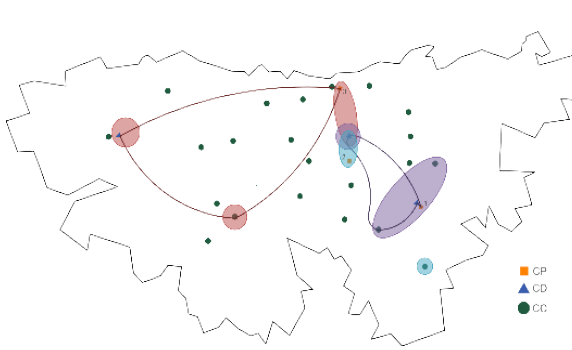
The routing model optimized the weight capacity utilization levels of the vehicles used in the trips in phase I, since it was noted that weight is the most constraining aspect of the vehicle's capacity. Routing was carried out by assessing the possibility of pooling the demands of several CCs which vehicle’s weight capacity was not exceeded, in case that vehicle’s capacity is exceeded and an electric vehicle is being used, the truck with the highest capacity is allocated in order to cover the largest number of DCs with the least amount of travel required. In this way, 5 routings were determined, from the sources; PC1, PC3, DC1, DC2 and DC3 to the different CCs whose trips had lower percentages of vehicle weight capacity utilization, therefore routing is performed with the last trip allocated for each CC. In Table 7, OTM mappings are observed with routing, where regions represent consumer centers whose deliveries are assigned to each PC or DC without routing and the lines indicate routing that is performed from sources, then supplying the demand of each of the consumer centers.
Table 7 Travel assignment for PCs and DCs.
| Assigning of trips from PCs | |
| |
| Source | Destination |
| PC1 | DC1, DC2, CC10 |
| PC2 | Does not perform routing |
| PC3 | DC3, CC2 |
| Assigning of trips from DCs | |
| |
| Source | Destination |
| DC1 | CC12, CC15 |
| DC2 | CC15, CC20, CC5, CC17, CC14, CC3, DC3, CC13, CC2, CC22, CC21, CC4, CC18, CC10 |
| DC3 | CC7, CC9, CC11, CC19 |
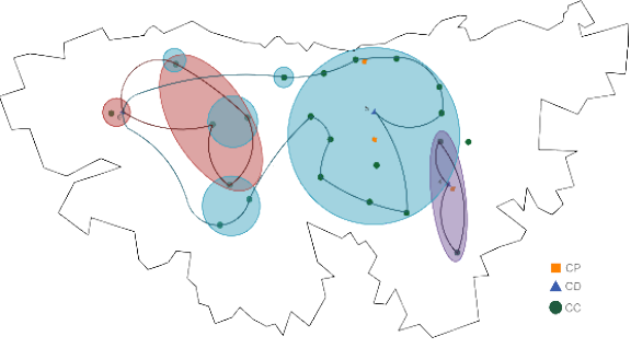
For the five routes shown in Table 7, the specific paths to follow are provided in blue for the PCs and DCs in Figures 3, 4 and 5, respectively, these were made through the Google Maps tool.
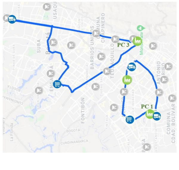
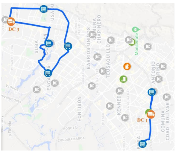
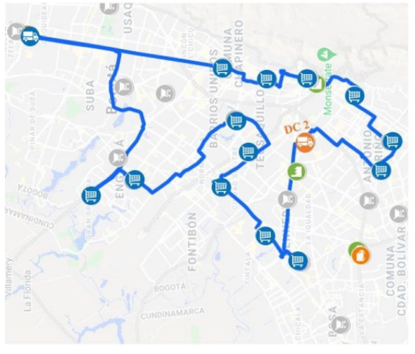
Table 8 shows the results of the routes, furthermore, it is noted that the truck type vehicle is used in routes from the PCs, and the electric type is used in routes from the DCs, except for routing from the DC2 which used a truck type vehicle due to the high number of CCs assigned to it. Moreover, the other indicators of time, distance, vehicle weight utilization and total cost of transport were also established.
Table 8 OTM Indicators with routing.
| Indicator | Result | ||||||
|---|---|---|---|---|---|---|---|
| Travel | Vehicle Type | Truck | Electric | ||||
| Source | PC1 | PC2 | PC3 | DC1 | DC2 | DC3 | |
| Amount | 2 | 2 | 2 | 2 | 13* | 7 | |
| Time (min) | 1242 | ||||||
| Distance to Distance (Km) | 599 | ||||||
| %Use | 84.7% | ||||||
| Total Transportation Cost (USD) | 945.2 | ||||||
*Of 13 trips, it is noted that 12 trips are assigned to the Electric vehicle and 1 trip is assigned to the truck.
7. Conclusions
A model that determined the allocation and routing for the weekly planning of the distribution of soda drink products for a company located in Bogota was obtained. Phase I (allocation) worked with two optimization models considering the capacity of the vehicles, costs of each trip and costs of transporting the units, establishing two important aspects: firstly, the models did not show significant differences in costs, since the OTM exceed CTM by at least 1% of the cost difference, however, there were differences in time and distance, where the CTM generated 18% more travel distance and 3% more time. Secondly, because of the company has two types of vehicles, the OTM relative to the CTM managed to reduce the travel of two electric vehicles by using an extra truck, despite the OTM had lower capacity usage rates than the CTM. In phase II, the use of a TSP model significantly improved indicators by defining travelling routes that had less than 25% use of the vehicle's capacity, improving the vehicles capacity usage and the delivery time of products to consumer centers at the same time. In conclusion, by addressing this problem through two phases, an initial solution to the entire system can be generated, assigning the trips established by the selected transshipment model, and then focusing on some specific cases where a better route allocation can be found from the TSP model.

