1. Introduction

This paper presents a real-life problem for the design of an opening hazardous material production and distribution network by optimizing capital expenditures (CAPEX) and operating expenses (OPEX). The problem presents a high degree of complexity, mostly because both CAPEX and OPEX play a major role in the feasibility of the venture. CAPEX includes buying machinery, acquiring permits, and investment in transport vehicles (fleet size), whereas OPEX involves a hazardous material to the customers (truck drivers and truck fuel) and the raw material costs.

The problem considers that a company has evaluated several locations on which to install the processing of a product and distribute from there to different customer’s locations. The transportation is considered as in-house, reason why the fleet size and vehicles capacities are a decision of the owners or investors of the company. The company business model requires the customers to sign a take-or-pay off contract in which it is obligated to pay for a specific amount of product independent on whether it is consumed or not. This business model allows for the planning of the whole contract period by the selection of supply stations, machinery and transport routes.

In this paper, a new version of the Multi Depot Multi Period Vehicle Routing Problem with heterogeneous fleet (MDMPVRPHF) is proposed. In this version, CAPEX are included to the MDMPVRPHF model as a set of restrictions that must be considered to design a better freight distribution network. We called this model the Multi Depot Multi Period Vehicle Routing Problem with heterogeneous fleet and management restrictions (MDMPVRPHFMR).

The MDMPVRPHF and the MDMPVRPHFMR are variants of the vehicle routing problem (VRP). The VRP is introduced by ^{Dantzig and Ramser (1959)}. It is the generalization of the Traveling Salesman Problem (TSP) presented by ^{Flood (1956)}. The classic VRP aims to design a network by minimizing distances, travel times or transportation costs. The network is defined on a graph

G = (V, Ɛ, C), where V = {V ₀ , …, V _n } is a set of vertices, Ɛ = {(V _i , V _j )│(V _i , V _j ) ϵ V ² , i ≠ j } is the arc set; and

C = (C _ij ) _{(Vi, Vj)ϵƐ} is a cost matrix defined over Ɛ. The depot is vertex V ₀ and the customers to be served are represented by the remaining vertices V (^{Pillac, Gendreau, Guéret, & Medaglia, 2013}). The classic VRP consists in designing a network by finding a set of routes for a fleet of vehicles with the same capacity, customer´s demands are known and supplied by only one vehicle (^{Archetti & Speranza, 2008}).

Different VRP variants have been developed. The most studied are the Capacitated VRP (CVRP), the VRP with time Windows (VRPTW), the VRP with Pick-up and Delivery (PDP), the Split Delivery Vehicle Routing Problem (SDVRP), and the Heterogeneous fleet VRP (HVRP).

In the CVRP, a set of customers have a different demand for a good and the fleet of vehicles have finite capacity (^{Pillac et al., 2013}). The VRPTW designs routes from one depot to a set of dispersed customers who can be supplied once by only one vehicle in a time interval, every route starts and ends at the depot, the total demand transported per route (sum of the demands of all points in a route) cannot exceed the capacity of the vehicle (^{Braysy & Gendreau, 2005}). In the PDP, a specific amount of goods must be picked-up and delivered to customers (^{Pillac et al., 2013}). Contrary to the classical VRP, the SDVRP does not consider the restriction that costumers that costumers are supplied by only one different capacities and costs is available for the distribution of goods (^{Baldacci, Battarra, & Vigo, 2008}).

In the literature, there are many variations of the HVRP problem with vehicles capacities constraints and with time window constraints to consider multiple depots, multiple trips to be operated by the vehicles, multiple vehicles with different capacities and other operational constraints. These HVRP variations are the Heterogeneous VRP with Fixed Costs and Vehicle Dependent Routing Costs (HVRPFD), the Heterogeneous VRP with Vehicle Dependent Routing Costs (HVRPD), the Fleet Size and Mix VRP with Fixed Costs and Vehicle Depending Routing Costs (FSMFD), the Fleet Size and Mix VRP with Vehicle Dependent Routing Costs (FSMD), the Fleet Size and Mix VRP with Fixed Costs (FSMF), and the Site-Dependent VRP (SDVRP) (^{Baldacci et al., 2008}).

^{Goel and Gruhn (2008)} study the VRP in real-life applications, and they find different difficulties to be considered. In real-life, the VRP must consider a heterogeneous fleet of vehicles, time window restrictions, differing travel times and costs, vehicles capacity, facility capacity, vehicle compatibility with specific orders, multiple pick-ups per order, delivery locations, service locations, orders where a vehicle can start and finish a journey at different locations, and vehicle route restrictions such as maximum sizes and weights. They include these difficulties as restrictions into the classic VRP and therefore, they formulate the General Vehicle Routing Problem (GVRP). Based on the GVRP, ^{Mancini (2016)} develops the MDMPVRPHF. In her study, Mancini explains that real-life cargo distribution problems have a high degree of complexity because of multi-dimensional vehicle capacity constraints, characteristics of the vehicles, route lengths and travel times, time windows, the compatibility between products, the compatibility between products and vehicles, the compatibility between customers and vehicles, and objective functions which consider different costs such as transportation costs, inventory costs, opportunity costs, etc.

In this article, the MDMPVRPHFMR recognizes the MDMPVRPHF restrictions and adds and proves that CAPEX transport vehicles) and OPEX (raw material cost and transportation of product to the customers such as truck drivers and truck fuel).

This article presents the application of the MDMPVRPHFMR to a real-life problem for the design of an opening liquefied natural gas (LNG) distribution network for a planning time horizon. In this study case, the CAPEX and OPEX information of a real company is used to design its distribution network prior to establishing a contract with the client. The model simultaneously optimizes location allocation, production capacity and vehicle routing decisions. To solve the problem, we present optimal solutions for different random variables small instances using the optimization software CPLEX from IBM. The customers’ demands and the distances between nodes (suppliers and customers) have been generated using Mersenne Twister which is a random number generator. These values are different for each instance and they are presented in Appendix A.

The paper is organized as follows. In Section 2, the MDMPVRPHF and the MDMPVRPHFMR problems are described and the mixed integer linear programming models are presented. In Section 3, the study case is presented together with the computing results of the application of the MDMPVRPHF and the MDMPVRPHFMR models. Section 4 presents the aleatory instances used to test the MDMPVRPHF and the MDMPVRPHFMR models and their computing results. Finally, conclusions and references are included.

2. MDMPVRPHFMR problem description and mathematical

3. Study case

In this Section, a real-life study case is presented to evaluate the performance of the proposed MDMPVRPHFMR model against the performance of the MDMPVRPHFMRWP model and the MDMPVRPHF model. For the real-life study case, the names of the locations are confidential and therefore not shown.

In this study case, the currency is USD and the input data is as follows: a contract period of 5 years, the maximum route travelling time α is equal to 10 [h], the vehicles average speed s is equal to 50 [km/h], the planning time horizon Θ is equal to 24 [h], the transport capacity per vehicle Cv is equal to 23,128 m3 of LNG, the cost of usage per vehicle μv is equal to 0.526 [$/km], the time to discharge/charge the hazardous material from the vehicle to each customer δj is equal to 0.5 [h], the penalty cost in time γ is 20 [$], the cost of renting/buying the vehicle βv is equal to 6.36 [$/h] and the machines production capacity of LNG cim is equal to 863.33 [m3/h].

The cost of opening the supply stations are shown in Table 1. This costs correspond to the legal paperwork and a physical installations needed to connect the station to a natural gas supply, which is the raw material. In the case of Supply Station 2 (SS_2), there is no cost because the client already has a connection to the natural gas pipe line. The supply station opening cost ρi for Supply Station 1 (SS_1) and Supply Station 3 (SS_3) for a 5-year contract period is ρ1=ρ3= 500,000 / (5*365) = 273.97 [$/day].

Table 2 shows the distance between nodes or between supply stations and customers in km. Where Customer 1 (C_1), Customer 2 (C_2) and Customer 3 (C_3) are three demand nodes for the same customer and SS_1, SS_2 and SS_3 are the three possible supplier stations.

The total amount of fuel consumed by the three demand nodes (C_1, C_2 and C_3) for a 5-year contract period is 412,836,900 [m3].

The customer demand nodes are shown in Table 3.

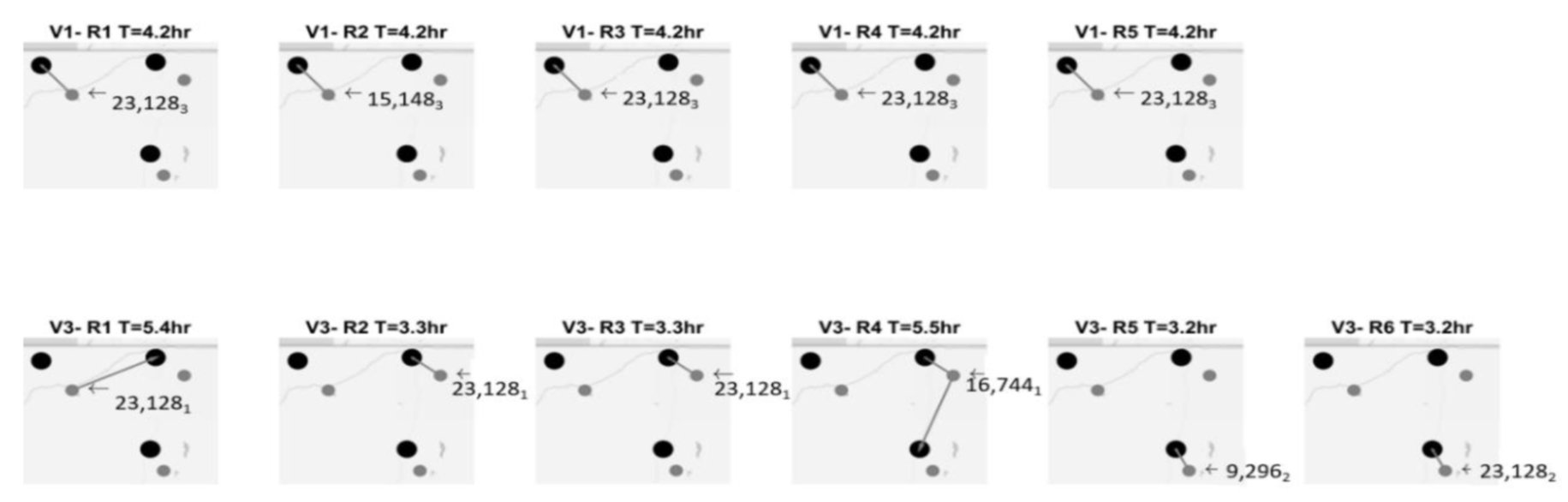
Fig. 1 shows the results for the application of the MDMPVRFHF model. In Fig. 1, Fig. 2 and Fig. 3, the dark circles indicate supply stations that are not part of the solution, the big dark dots indicate the supply stations that are part of the solution, the little light dots indicate the customer locations and the medium size dots indicate the customer locations where LNG is delivered. Each row corresponds to a vehicle v∈V whereas the columns correspond to the route k∈K. Each route has a title, e.g. “V1-R2 T=5.5h” with the following notation: “V” corresponds to the vehicle, “R” corresponds to the route, “T” corresponds to the time of the route. Vehicle routes are consecutive, it means “R1” happens before “R2”, and so on. The quantity delivered of LNG is indicated by the number with an arrow pointing to its location in [m3]. The subscript of the quantity delivered corresponds to the supply station number where that quantity is produced.

Fig. 1. Transport routes of the solution obtained with the MDMPVRFHF model. 

Fig. 2. Transport routes of the solution obtained with the MDMPVRFHFMRWP model. 

Fig. 3. Transport routes of the solution obtained with the MDMPVRFHFMR model. 

The production needed in SS_1, SS_2 and SS_3 to satisfy the customer demands at C_1, C_2 and C_3 are shown in Table 4.

The transport routes using the MDMPVRFHF model are shown in Fig. 1. Vehicle 1 (V1) operates five routes per day and vehicle 2 (V2) operates six routes per day.

Although, in the MDMPVRFHF model only TRA and VEH are minimized, all CAPEX and OPEX costs are considered for the calculation of the customers fuel priceas shown in Table 5.

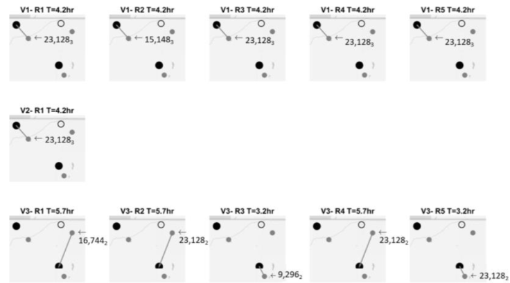
The transport routes using the MDMPVRFHFMRWP model are shown in Fig. 2. Vehicle 1 (V1) operates five routes per day, vehicle 2 (V2) operates one route per day, and vehicle 3 (V3) operates five routes per day. The production needed in SS_2 and SS_3 to satisfy the customer demands at C_1, C_2 and C_3 are shown in Table 6. The results indicate that SS_1 is not required to operate, therefore there are no opening costs for this station.

Table 7 shows all the costs considered for the customer’s fare when using the MDMPVRFHFMRWP model. By comparing the total cost per m3 of LNG from Table 5 and Table 7, it is possible to conclude that the total cost is reduced from $0.24786 to $0.23893 USD. The results demonstrate that the MDMPVRFHFMRWP model achieves lower costs than the MDMPVRFHF model.

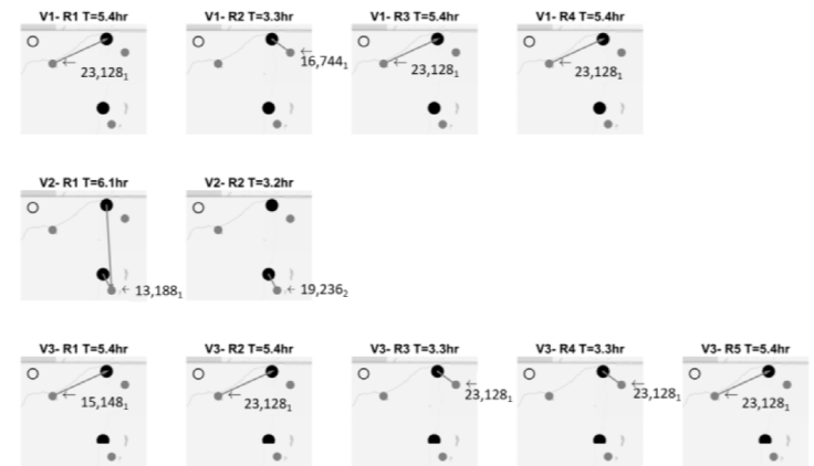
Finally, the transport routes using the MDMPVRFHFMR model are shown in Fig. 3. Vehicle 1 (V1) operates four routes per day, vehicle 2 (V2) operates two routes per day, and vehicle 3 (V3) operates five routes per day. The production needed in SS_1 and SS_2 to satisfy the customer demands at C_1, C_2 and C_3 are shown in Table 8. The results indicate that SS_3 is not required to operate, therefore there are no opening costs for this station.

Table 9 shows all the costs considered for the customer’s fare when using the MDMPVRFHFMR model. By comparing the total cost per m3 of LNG from Table 5 ($0.24786), Table 7 ($0.23893), and Table 9 ($0.23), it is possible to conclude that the minimum total cost, and hence the minimum fuel price (Sj), is reached when using the MDMPVRFHFMR model. Therefore, the results obtained with the proposed MDMPVRFHFMR model indicates that TRA, VEH, PEN, RAX, INV, and MCH costs must be considered. It also demonstrates that the model proposed by ^{Mancini (2016)} (the MDMPVRFHFMR model) does not achieve the lowest possible cost.

The best fuel price for the customer (S _j ) is obtained when using the proposed MDMPVRFHFMR model. It is important to notice that the machine utilization increases when we consider the MCH. The unitary costs TRA, VEH and INV for the three models are compared in Fig. 4. The unitary costs RAW, MCH and the sum of all costs are compared in Fig. 5 for the three models under study.

Fig. 4 The RAW, MCH and the total costs for the MDMPVRPHF model. 

Fig. 5 The TRA, VEH and VEH costs for the MDMPVRPHF model. 

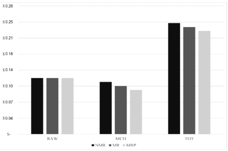
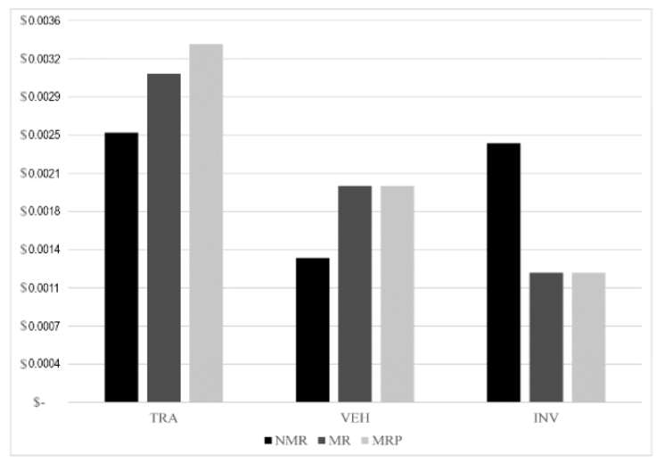
Although OPEX increases when all costs are minimized, the MCH costs decreases and therefore the total cost is minimized and the best fuel price for the customer (S _j ) is obtained.

4. Computational Results

In this section, we test the performance of the MDMPVRPHF model, the MDMPVRPHFMRWP model, and the MDMPVRPHFMR model. These tests study how suitable the models are to solve small and medium instances. A description of the instances used in the computational study is given in Appendix A. Table 10 shows the computation results for each instance tested.

Fig. 6 shows the relative gap between the upper and lower bounds. Here, it is possible to conclude that the MDMPVRPHFMR model achieves the lowest relative gap in the same amount of computing time. For solving the MDMPVRPHFMRWP, the relative gap increases probably because the MDMPVRPHF does not narrow the possible best solutions. In the case of the MDMPVRPHFMR model, OPEX and CAPEX narrows the feasible solutions region.

Fig. 6. Relative gap for instances with 15 and 20 demand points. 

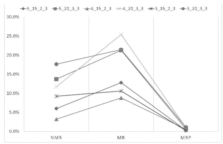
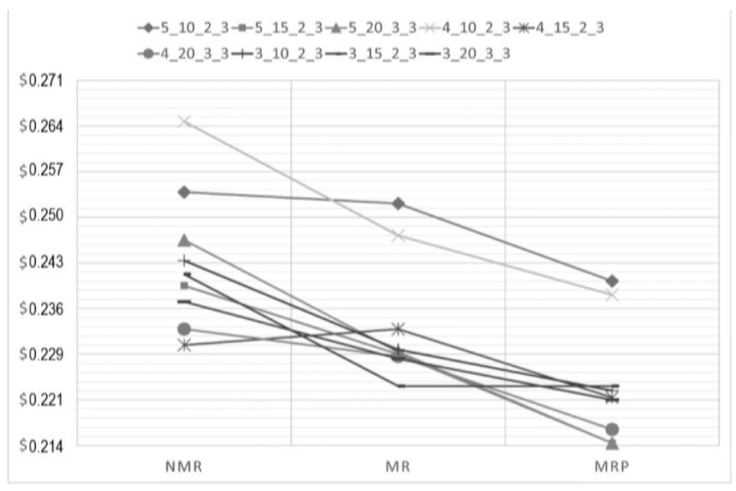
Fig. 7 shows the LNG fuel prices with the MDMPVRPHF model, the MDMPVRPHFMRWP model and the MDMPVRPHFMR model. The LNG fuel price are minimized for all instances when using the MDMPVRPHFMR model. Therefore, we can conclude that companies must consider CAPEX and OPEX for designing their supply chain networks when the contract period is fixed between the supplier and the customer.

Fig. 7. Fuel cost for instances with 10, 15 and 20 demand points. 

5. Conclusions and Future Work

The Multi Depot Multi Period Vehicle Routing Problem with heterogeneous fleet and management restrictions (MDMPVRPHFMR) has been introduced and formulated in this paper. This is a modification of ^{Mancini (2016)} Multi Depot Multi Period Vehicle Routing Problem with heterogeneous fleet (MDMPVRPHF) to consider capital expenditures and operating expenses (MDMPVRPHFMR). In the MDMPVRPHFMR, the goal is to carry out delivery operations at the minimum costs by considering transport costs, vehicle rent costs, time services, raw material, investments, and machine costs. In this paper, we test the proposed MDMPVRPHFMR model and the MDMPVRPHF model in a real case scenario and by solving different instances with random parameters to test the effectiveness and efficacy of these models. The results allows to compare the performance of the proposed MDMPVRPHFMR model with the results obtained using the model proposed by ^{Mancini (2016)} or MDMPVRPHF model. By comparing results, it is possible to conclude that the minimum total cost, and hence the minimum fuel price (Sj), is reached when using the MDMPVRFHFMR model. The results indicates that CAPEX and OPEX must be considered. It also demonstrates that the model proposed by ^{Mancini (2016)} (the MDMPVRFHFMR model) does not achieve the lowest possible cost in a real company scenario.

The major contribution of this paper is the proposition of a model capable of minimizing CAPEX and OPEX at the same time with the aim of designing a LNG supply chain network considering must of the variables presented in a real company scenario. By considering more variables and having more real restrictions the feasible solutions region is narrowed and therefore the relative gap between the upper and lower bound is reduced. Finally, it is possible to conclude that companies must consider CAPEX and OPEX for designing real supply chain networks when the contract period is fixed between the supplier and the customer.

As future work, a Periodic Multi Period Vehicle Routing Problem with heterogeneous fleet and management restrictions can be developed for companies that require periodic deliveries. Such a model can be an extension of the periodic vehicle routing problem (PVRP) and the MDMPVRPHFMR.

References

Archetti, C., & Speranza, M. G. (2008). The Split Delivery Vehicle Routing Problem: A Survey. Operations Research / Computer Science Interfaces, 43, 103-122. [ Links ]
Baldacci, R., Battarra, M., & Vigo, D. (2008). Routing a Heterogeneous Fleet of Vehicles. Latest Advances and New Challenges. Operations Research/Computer Science Interfaces, 43, 3-27. [ Links ]
Braysy, O., & Gendreau, M. (2005). Vehicle Routing Problem with Time Windows, Part I: Route Construction and Local Search Algorithms. Transportation Science, 39(1), 104-118. [ Links ]
Coelho, L. C., & Laporte, G. (2013). The exact solution of several classes of inventory-routing problems. Computers & Operations Research, 40(2), 558-565. [ Links ]
Current, J., Ratick, S., & Revelle, C. (1997). Dynamic facility location when the total number of facilities is uncertain: A decision analysis approach. European Journal of Operational Research, 110(3), 597-609. [ Links ]
Dantzig, G., & Ramser, J. (1959). The truck dispatching problem. Management Science, 6(1), 80-91. [ Links ]
Flood, M. (1956). The traveling-salesman problem. Operations Research, 4(1), 61-75. [ Links ]
Goel, A., & Gruhn, V. (2008). A General Vehicle Routing Problem. European Journal of Operational Research, 191(3), 650-660. [ Links ]
Mancini, S. (2016). A real-life Multi Depot Multi Period Vehicle Routing Problem with a Heterogeneous Fleet: Formulation and Adaptive Large Neighborhood Search based Metaheuristics. Transport Research Part C: Emerging Technologies, 70, 100-112. [ Links ]
Miranda P. A., & Garrido, R. A. (2004). Incorporating inventory control decisions into a strategic distribution network design model with stochastic demand. Transportation Research Part E: Logistics and Transportation Review, 40(3), 183-207. [ Links ]
Owen, S. H., & Daskin, M. S. (1998). Strategic facility location: A review. European Journal of Operational Research, 111, 423-447. [ Links ]
Pillac, V., Gendreau, M., Guéret, C., & Medaglia, A. L. (2013). A review of dynamic vehicle routing problems. European Journal of Operational Research, 225(1), 1-11. [ Links ]
Vidal, C. J., & Goetschalckx, M. (1997). Strategic production-distribution models: A critical review with emphasis on global supply chain models. European Journal of Operational Research, 98(1), 1-18. [ Links ]
Appendix A.
All instances have the parameters shown in Table A.1.
Table A.1. Fixed parameters for all instances.
Description Variable Value Unit
• Contract period
• Maximum route duration
• Vehicles average speed
• Planning time horizon
• Transport capacity per vehicle
• Cost of usage per vehicle
• Machine cost
• Production capacity of machine
• Time to discharge/charge material
• Penalty cost in visit times
• Cost of renting/buying the vehicle
• -
• α
• s
• Θ
• C v
• μ v
• p m
• c m
• δ i
• γ
• β
• 7
• 24
• 50
• 23,128
• $ 0.50
• $ 1,447.70
• 20,720
• 60
• 20
• 150
• [year]
• [h]
• [km/h]
• [m3]
• [$/km]
• [$/day]
• [m3/day]
• [$]
Instance 3_10_2_3:
Table A.2. General information of instance.
• No. of possible supply stations
• No. of demand locations
• No. of vehicles
• No. of routes
• No. of machines
• I
• D
• V
• K
• M
• 3
• 10
• 2
• 1
• [-]
Table A.3. Daily demand, opening costs and raw material cost of instance.
Location Demand [m3/day] Supply Station Opening cost [$/day] Raw material cost [$/m3]
C_1 11,760 SS_1 195.69 0.1464
C_2 3,500 SS_2 195.69 0.1429
C_3 6,776 SS_3 195.69 0.1393
C_4 10,332
C_5 11,480
C_6 1,624
C_7 13,468
C_8 10,024
C_9 3,892
C_10 6,076
Table A.4. Distance matrix for instance.
[km] C_1 C_3 C_3 C_4 C_5 C_6 C_7 C_8 C_9 C_10 SS_1 SS_2 SS_3
C_1 0 150 43 173 152 191 25 124 151 121 32 75 105
C_2 150 0 137 136 170 157 100 19 180 100 9 9 136
C_3 43 137 0 50 11 60 124 48 146 56 181 138 28
C_4 173 136 50 0 94 31 117 49 82 131 27 147 172
C_5 152 170 11 94 0 46 7 147 191 40 28 80 33
C_6 191 157 60 31 46 0 170 66 186 80 35 66 153
C_7 25 100 124 117 7 170 0 24 60 63 122 179 12
C_8 124 19 48 49 147 66 24 0 119 139 43 50 118
C_9 151 180 146 82 191 186 60 119 0 19 104 63 35
C_10 121 100 56 131 40 80 63 139 19 0 198 82 146
SS_1 32 9 181 27 28 35 122 43 104 198 0 142 107
SS_2 75 9 138 147 80 66 179 50 63 82 142 0 184
SS_3 105 136 28 172 33 153 12 118 35 146 107 184 0
Instance 3_15_2_3:
Table A.5. General information of instance.
• 15
Table A.6. Daily demand, opening costs and raw material cost of instance.
C_2 2,688 SS_2 195.69 0.1429
C_3 3,388 SS_3 195.69 0.1393
C_4 6,776
C_5 10,332
C_6 3,108
C_7 13,020
C_8 7,532
C_9 11,480
C_10 1,624
C_11 7,448
C_12 13,468
C_13 10,024
C_14 3,892
C_15 6,076
Table A.7. Distance matrix for instance.
[km] C_1 C_2 C_3 C_4 C_5 C_6 C_7 C_8 C_9 C_10 C_11 C_12 C_13 C_14 C_15 SS_1 SS_2 SS_3
C_1 0 124 154 43 173 56 141 124 152 191 181 25 124 151 121 32 75 105
C_2 124 0 149 67 199 118 195 193 157 42 150 28 14 86 104 57 36 149
C_3 154 149 0 46 41 193 195 150 23 156 53 67 28 54 168 111 26 15
C_4 43 67 46 0 50 105 81 52 11 60 25 124 48 146 56 181 138 28
C_5 173 199 41 50 0 19 127 193 94 31 39 117 49 82 131 27 147 172
C_6 56 118 193 105 19 0 198 109 66 170 30 140 21 188 184 167 88 40
C_7 141 195 195 81 127 198 0 7 127 157 118 6 172 52 102 161 76 122
C_8 124 193 150 52 193 109 7 0 47 55 15 106 140 107 195 184 196 109
C_9 152 157 23 11 94 66 127 47 0 46 165 7 147 191 40 28 80 33
C_10 191 42 156 60 31 170 157 55 46 0 99 170 66 186 80 35 66 153
C_11 181 150 53 25 39 30 118 15 165 99 0 50 133 14 85 116 63 85
C_12 25 28 67 124 117 140 6 106 7 170 50 0 24 60 63 122 179 12
C_13 124 14 28 48 49 21 172 140 147 66 133 24 0 119 139 43 50 118
C_14 151 86 54 146 82 188 52 107 191 186 14 60 119 0 19 104 63 35
C_15 121 104 168 56 131 184 102 195 40 80 85 63 139 19 0 198 82 146
SS_1 32 57 111 181 27 167 161 184 28 35 116 122 43 104 198 0 142 107
SS_2 75 36 26 138 147 88 76 196 80 66 63 179 50 63 82 142 0 184
SS_3 105 149 15 28 172 40 122 109 33 153 85 12 118 35 146 107 184 0
Instance 3_20_3_3:
Table A.8. General information of instance.
Table A.9. Daily demand, opening costs and raw material cost of instance.
C_2 9,184 SS_2 195.69 0.1429
C_3 2,688 SS_3 195.69 0.1393
C_4 3,388
C_5 1,624
C_6 3,500
C_7 6,776
C_8 10,332
C_9 3,108
C_10 13,020
C_11 7,532
C_12 11,480
C_13 2,492
C_14 6,468
C_15 1,624
C_16 7,448
C_17 13,468
C_18 10,024
C_19 3,892
C_20 6,076
Table A.10. Distance matrix for instance.
[km] C_1 C_2 C_3 C_4 C_5 C_6 C_7 C_8 C_9 C_10 C_11 C_12 C_13 C_14 C_15 C_16 C_17 C_18 C_19 C_20 SS_1 SS_2 SS_3
C_1 0 139 124 154 152 150 43 173 56 141 124 152 11 59 191 181 25 124 151 121 32 75 105
C_2 139 0 187 47 121 26 80 123 125 76 114 121 44 36 15 182 184 15 112 23 1 166 87
C_3 124 187 0 149 172 165 67 199 118 195 193 157 92 186 42 150 28 14 86 104 57 36 149
C_4 154 47 149 0 198 6 46 41 193 195 150 23 192 14 156 53 67 28 54 168 111 26 15
C_5 152 121 172 198 0 83 188 166 18 129 133 196 159 117 183 138 180 158 151 185 175 176 170
C_6 150 26 165 6 83 0 137 136 101 173 105 170 91 128 157 27 100 19 180 100 9 9 136
C_7 43 80 67 46 188 137 0 50 105 81 52 11 67 131 60 25 124 48 146 56 181 138 28
C_8 173 123 199 41 166 136 50 0 19 127 193 94 12 173 31 39 117 49 82 131 27 147 172
C_9 56 125 118 193 18 101 105 19 0 198 109 66 149 12 170 30 140 21 188 184 167 88 40
C_10 141 76 195 195 129 173 81 127 198 0 7 127 102 164 157 118 6 172 52 102 161 76 122
C_11 124 114 193 150 133 105 52 193 109 7 0 47 40 106 55 15 106 140 107 195 184 196 109
C_12 152 121 157 23 196 170 11 94 66 127 47 0 86 139 46 165 7 147 191 40 28 80 33
C_13 11 44 92 192 159 91 67 12 149 102 40 86 0 43 65 145 166 131 54 23 101 89 2
C_14 59 36 186 14 117 128 131 173 12 164 106 139 43 0 166 186 68 104 51 60 81 32 155
C_15 191 15 42 156 183 157 60 31 170 157 55 46 65 166 0 99 170 66 186 80 35 66 153
C_16 181 182 150 53 138 27 25 39 30 118 15 165 145 186 99 0 50 133 14 85 116 63 85
C_17 25 184 28 67 180 100 124 117 140 6 106 7 166 68 170 50 0 24 60 63 122 179 12
C_18 124 15 14 28 158 19 48 49 21 172 140 147 131 104 66 133 24 0 119 139 43 50 118
C_19 151 112 86 54 151 180 146 82 188 52 107 191 54 51 186 14 60 119 0 19 104 63 35
C_20 121 23 104 168 185 100 56 131 184 102 195 40 23 60 80 85 63 139 19 0 198 82 146
SS_1 32 1 57 111 175 9 181 27 167 161 184 28 101 81 35 116 122 43 104 198 0 142 107
SS_2 75 166 36 26 176 9 138 147 88 76 196 80 89 32 66 63 179 50 63 82 142 0 184
SS_3 105 87 149 15 170 136 28 172 40 122 109 33 2 155 153 85 12 118 35 146 107 184 0
Instance 3_25_4_4:
Table A.11. General information of instance.
• 25
• 4
Table A.12. Daily demand, opening costs and raw material cost of instance.
C_1 2,352 SS_1 195.69 0.1464
C_2 5,880 SS_2 195.69 0.1429
C_3 1,484 SS_3 195.69 0.1393
C_4 4,424
C_5 10,220
C_7 1,876
C_8 6,244
C_9 1,624
C_10 7,448
C_11 4,424
C_12 9,492
C_13 1,624
C_14 7,448
C_15 5,264
C_16 952
C_17 7,588
C_18 3,948
C_19 6,748
C_20 9,604
C_21 2,940
C_22 8,540
C_23 4,592
C_24 7,168
C_25 1,876
Table A.13. Distance matrix for instance.
[km] C_1 C_2 C_3 C_4 C_5 C_6 C_7 C_8 C_9 C_10 C_11 C_12 C_13 C_14 C_15 C_16 C_17 C_18 C_19 C_20 C_21 C_22 C_23 C_24 C_25 SS_1 SS_2 SS_3
C_1 0 28 188 119 60 56 43 22 12 58 135 176 167 49 30 24 136 20 41 91 7 61 23 145 79 107 157 133
C_2 28 0 28 118 52 68 77 88 92 14 131 200 146 167 182 77 11 147 104 129 67 194 183 134 148 115 114 71
C_3 188 28 0 134 178 58 6 57 145 17 107 173 106 163 129 163 161 128 11 27 150 180 97 36 196 83 163 70
C_4 119 118 134 0 90 35 95 198 68 14 144 8 166 126 33 49 136 15 173 91 129 39 171 111 105 3 116 51
C_5 60 52 178 90 0 80 67 122 81 82 101 109 103 1 114 177 190 25 89 131 34 1 162 192 86 141 189 191
C_6 56 68 58 35 80 0 196 51 106 25 98 200 111 76 187 143 19 197 110 166 191 143 38 120 42 102 175 60
C_7 43 77 6 95 67 196 0 27 179 89 100 103 43 181 157 76 182 100 114 62 109 174 50 162 65 77 102 32
C_8 22 88 57 198 122 51 27 0 156 180 188 175 118 137 138 50 102 5 137 81 51 24 11 197 23 13 158 73
C_9 12 92 145 68 81 106 179 156 0 71 78 15 29 76 94 51 123 11 75 177 116 8 122 178 76 72 95 149
C_10 58 14 17 14 82 25 89 180 71 0 24 198 11 127 53 154 64 29 16 141 184 120 156 43 66 47 166 142
C_11 135 131 107 144 101 98 100 188 78 24 0 185 137 49 114 10 16 179 92 49 180 121 103 7 69 41 65 141
C_12 176 200 173 8 109 200 103 175 15 198 185 0 122 115 50 138 171 94 10 152 97 104 6 91 164 163 196 2
C_13 167 146 106 166 103 111 43 118 29 11 137 122 0 197 64 125 29 113 148 59 89 2 199 3 107 79 56 75
C_14 49 167 163 126 1 76 181 137 76 127 49 115 197 0 183 150 75 99 8 56 63 138 101 95 105 11 15 181
C_15 30 182 129 33 114 187 157 138 94 53 114 50 64 183 0 196 125 14 191 2 12 190 67 191 155 76 151 64
C_16 24 77 163 49 177 143 76 50 51 154 10 138 125 150 196 0 200 180 149 75 151 175 35 50 25 155 167 120
C_17 136 11 161 136 190 19 182 102 123 64 16 171 29 75 125 200 0 58 188 88 27 23 126 78 126 34 185 60
C_18 20 147 128 15 25 197 100 5 11 29 179 94 113 99 14 180 58 0 103 61 72 71 116 87 70 183 66 26
C_19 41 104 11 173 89 110 114 137 75 16 92 10 148 8 191 149 188 103 0 59 80 49 151 167 67 64 161 78
C_20 91 129 27 91 131 166 62 81 177 141 49 152 59 56 2 75 88 61 59 0 178 113 31 165 115 66 108 164
C_21 7 67 150 129 34 191 109 51 116 184 180 97 89 63 12 151 27 72 80 178 0 123 72 91 173 41 93 197
C_22 61 194 180 39 1 143 174 24 8 120 121 104 2 138 190 175 23 71 49 113 123 0 29 77 40 154 165 173
C_23 23 183 97 171 162 38 50 11 122 156 103 6 199 101 67 35 126 116 151 31 72 29 0 186 135 14 191 17
C_24 145 134 36 111 192 120 162 197 178 43 7 91 3 95 191 50 78 87 167 165 91 77 186 0 181 191 16 68
C_25 79 148 196 105 86 42 65 23 76 66 69 164 107 105 155 25 126 70 67 115 173 40 135 181 0 32 142 48
SS_1 107 115 83 3 141 102 77 13 72 47 41 163 79 11 76 155 34 183 64 66 41 154 14 191 32 0 47 64
SS_2 157 114 163 116 189 175 102 158 95 166 65 196 56 15 151 167 185 66 161 108 93 165 191 16 142 47 0 110
SS_3 133 71 70 51 191 60 32 73 149 142 141 2 75 181 64 120 60 26 78 164 197 173 17 68 48 64 110 0
Instance 4_10_2_3:
Table A.14. General information of instance.
Table A.15. Daily demand, opening costs and raw material cost of instance.
C_1 3,388 SS_1 195.69 0.1357
C_2 13,020 SS_2 195.69 0.1393
C_3 2,492 SS_3 195.69 0.1429
C_4 6,468 SS_4 195.69 0.1464
C_6 4,424
Table A.16. Distance matrix for instance.
[km] C_1 C_2 C_3 C_4 C_5 C_6 C_7 C_8 C_9 C_10 SS_1 SS_2 SS_3 SS_4
• C_1
• C_2
• C_3
• C_4
• C_5
• C_6
• C_7
• C_8
• C_9
• C_10
• SS_1
• SS_2
• SS_3
• SS_4
• 0
• 195
• 192
• 14
• 156
• 53
• 67
• 28
• 54
• 168
• 111
• 26
• 43
• 102
• 164
• 157
• 118
• 6
• 172
• 52
• 161
• 76
• 84
• 122
• 65
• 145
• 166
• 131
• 23
• 101
• 89
• 186
• 68
• 104
• 51
• 81
• 32
• 155
• 99
• 170
• 66
• 80
• 35
• 94
• 153
• 133
• 85
• 116
• 63
• 179
• 87
• 12
• 119
• 139
• 141
• 19
• 198
• 82
• 37
• 146
• 142
• 107
• 75
• 184
• 152
Instance 4_15_2_3:
Table A.17. General information of instance.
No. of possible supply stations I 4 [-]
No. of demand locations D 15 [-]
No. of vehicles V 2 [-]
No. of routes K 3 [-]
No. of machines M 1 [-]
Table A.18. Daily demand, opening costs and raw material cost of instance.
C_1 11,844 SS_1 195.69 0.1357
C_2 3,388 SS_2 195.69 0.1393
C_3 7,168 SS_3 195.69 0.1429
C_4 6,776 SS_4 195.69 0.1464
C_5 13,020
C_6 7,532
C_7 11,480
C_8 2,492
C_9 6,468
Table A.19. Distance matrix for instance.
[km] C_1 C_2 C_3 C_4 C_5 C_6 C_7 C_8 C_9 C_10 C_11 C_12 C_13 C_14 C_15 SS_1 SS_2 SS_3 SS_4
C_1 0 47 26 80 76 114 121 44 36 15 182 184 15 112 23 1 166 151 87
C_2 47 0 6 46 195 150 23 192 14 156 53 67 28 54 168 111 26 43 15
C_3 26 6 0 137 173 105 170 91 128 157 27 100 19 180 100 9 9 112 136
C_4 80 46 137 0 81 52 11 67 131 60 25 124 48 146 56 181 138 171 28
C_5 76 195 173 81 0 7 127 102 164 157 118 6 172 52 102 161 76 84 122
C_6 114 150 105 52 7 0 47 40 106 55 15 106 140 107 195 184 196 72 109
C_7 121 23 170 11 127 47 0 86 139 46 165 7 147 191 40 28 80 98 33
C_8 44 192 91 67 102 40 86 0 43 65 145 166 131 54 23 101 89 52 2
C_9 36 14 128 131 164 106 139 43 0 166 186 68 104 51 60 81 32 186 155
C_10 15 156 157 60 157 55 46 65 166 0 99 170 66 186 80 35 66 94 153
C_11 182 53 27 25 118 15 165 145 186 99 0 50 133 14 85 116 63 51 85
C_12 184 67 100 124 6 106 7 166 68 170 50 0 24 60 63 122 179 87 12
C_13 15 28 19 48 172 140 147 131 104 66 133 24 0 119 139 43 50 141 118
C_14 112 54 180 146 52 107 191 54 51 186 14 60 119 0 19 104 63 81 35
C_15 23 168 100 56 102 195 40 23 60 80 85 63 139 19 0 198 82 37 146
SS_1 1 111 9 181 161 184 28 101 81 35 116 122 43 104 198 0 142 172 107
SS_2 166 26 9 138 76 196 80 89 32 66 63 179 50 63 82 142 0 75 184
SS_3 151 43 112 171 84 72 98 52 186 94 51 87 141 81 37 172 75 0 152
SS_4 87 15 136 28 122 109 33 2 155 153 85 12 118 35 146 107 184 152 0
Instance 4_20_3_3:
Table A.20. General information of instance.
Table A.21. Daily demand, opening costs and raw material cost of instance.
Location Demand[m3/day] Supply Station Opening cost [$/day] Raw material cost [$/m3]
C_1 9,856 SS_1 195.69 0.1357
C_2 11,844 SS_2 195.69 0.1393
C_3 2,688 SS_3 195.69 0.1429
C_4 3,388 SS_4 195.69 0.1464
C_6 7,168
C_16 4,424
Table A.22. Distance matrix for instance.
[km] C_1 C_2 C_3 C_4 C_5 C_6 C_7 C_8 C_9 C_10 C_11 C_12 C_13 C_14 C_15 C_16 C_17 C_18 C_19 C_20 SS_1 SS_2 SS_3 SS_4
C_1 0 139 124 154 152 150 43 173 56 141 124 152 11 59 191 181 25 124 151 121 32 75 7 105
C_2 139 0 187 47 121 26 80 123 125 76 114 121 44 36 15 182 184 15 112 23 1 166 151 87
C_3 124 187 0 149 172 165 67 199 118 195 193 157 92 186 42 150 28 14 86 104 57 36 141 149
C_4 154 47 149 0 198 6 46 41 193 195 150 23 192 14 156 53 67 28 54 168 111 26 43 15
C_5 152 121 172 198 0 83 188 166 18 129 133 196 159 117 183 138 180 158 151 185 175 176 136 170
C_6 150 26 165 6 83 0 137 136 101 173 105 170 91 128 157 27 100 19 180 100 9 9 112 136
C_7 43 80 67 46 188 137 0 50 105 81 52 11 67 131 60 25 124 48 146 56 181 138 171 28
C_8 173 123 199 41 166 136 50 0 19 127 193 94 12 173 31 39 117 49 82 131 27 147 112 172
C_9 56 125 118 193 18 101 105 19 0 198 109 66 149 12 170 30 140 21 188 184 167 88 181 40
C_10 141 76 195 195 129 173 81 127 198 0 7 127 102 164 157 118 6 172 52 102 161 76 84 122
C_11 124 114 193 150 133 105 52 193 109 7 0 47 40 106 55 15 106 140 107 195 184 196 72 109
C_12 152 121 157 23 196 170 11 94 66 127 47 0 86 139 46 165 7 147 191 40 28 80 98 33
C_13 11 44 92 192 159 91 67 12 149 102 40 86 0 43 65 145 166 131 54 23 101 89 52 2
C_14 59 36 186 14 117 128 131 173 12 164 106 139 43 0 166 186 68 104 51 60 81 32 186 155
C_15 191 15 42 156 183 157 60 31 170 157 55 46 65 166 0 99 170 66 186 80 35 66 94 153
C_16 181 182 150 53 138 27 25 39 30 118 15 165 145 186 99 0 50 133 14 85 116 63 51 85
C_17 25 184 28 67 180 100 124 117 140 6 106 7 166 68 170 50 0 24 60 63 122 179 87 12
C_18 124 15 14 28 158 19 48 49 21 172 140 147 131 104 66 133 24 0 119 139 43 50 141 118
C_19 151 112 86 54 151 180 146 82 188 52 107 191 54 51 186 14 60 119 0 19 104 63 81 35
C_20 121 23 104 168 185 100 56 131 184 102 195 40 23 60 80 85 63 139 19 0 198 82 37 146
SS_1 32 1 57 111 175 9 181 27 167 161 184 28 101 81 35 116 122 43 104 198 0 142 172 107
SS_2 75 166 36 26 176 9 138 147 88 76 196 80 89 32 66 63 179 50 63 82 142 0 75 184
SS_3 7 151 141 43 136 112 171 112 181 84 72 98 52 186 94 51 87 141 81 37 172 75 0 152
SS_4 105 87 149 15 170 136 28 172 40 122 109 33 2 155 153 85 12 118 35 146 107 184 152 0
Instance 4_25_4_4:
Table A.23. General information of instance.
Table A.24. Daily demand, opening costs and raw material cost of instance.
C_1 2,352 SS_1 195.69 0.1357
C_2 5,880 SS_2 195.69 0.1393
C_3 1,484 SS_3 195.69 0.1429
C_4 4,424 SS_4 195.69 0.1464
Table A.25. Distance matrix for instance.
[km] C_1 C_2 C_3 C_4 C_5 C_6 C_7 C_8 C_9 C_10 C_11 C_12 C_13 C_14 C_15 C_16 C_17 C_18 C_19 C_20 C_21 C_22 C_23 C_24 C_25 SS_1 SS_2 SS_3 SS_4
C_1 0 28 188 119 60 56 43 22 12 58 135 176 167 49 30 24 136 20 41 91 7 61 23 145 79 107 186 130 133
C_2 28 0 28 118 52 68 77 88 92 14 131 200 146 167 182 77 11 147 104 129 67 194 183 134 148 115 147 141 71
C_3 188 28 0 134 178 58 6 57 145 17 107 173 106 163 129 163 161 128 11 27 150 180 97 36 196 83 150 187 70
C_4 119 118 134 0 90 35 95 198 68 14 144 8 166 126 33 49 136 15 173 91 129 39 171 111 105 3 82 138 51
C_5 60 52 178 90 0 80 67 122 81 82 101 109 103 1 114 177 190 25 89 131 34 1 162 192 86 141 48 114 191
C_6 56 68 58 35 80 0 196 51 106 25 98 200 111 76 187 143 19 197 110 166 191 143 38 120 42 102 105 77 60
C_7 43 77 6 95 67 196 0 27 179 89 100 103 43 181 157 76 182 100 114 62 109 174 50 162 65 77 44 127 32
C_8 22 88 57 198 122 51 27 0 156 180 188 175 118 137 138 50 102 5 137 81 51 24 11 197 23 13 169 73 73
C_9 12 92 145 68 81 106 179 156 0 71 78 15 29 76 94 51 123 11 75 177 116 8 122 178 76 72 133 82 149
C_10 58 14 17 14 82 25 89 180 71 0 24 198 11 127 53 154 64 29 16 141 184 120 156 43 66 47 164 74 142
C_11 135 131 107 144 101 98 100 188 78 24 0 185 137 49 114 10 16 179 92 49 180 121 103 7 69 41 159 94 141
C_12 176 200 173 8 109 200 103 175 15 198 185 0 122 115 50 138 171 94 10 152 97 104 6 91 164 163 94 101 2
C_13 167 146 106 166 103 111 43 118 29 11 137 122 0 197 64 125 29 113 148 59 89 2 199 3 107 79 62 183 75
C_14 49 167 163 126 1 76 181 137 76 127 49 115 197 0 183 150 75 99 8 56 63 138 101 95 105 11 138 42 181
C_15 30 182 129 33 114 187 157 138 94 53 114 50 64 183 0 196 125 14 191 2 12 190 67 191 155 76 198 68 64
C_16 24 77 163 49 177 143 76 50 51 154 10 138 125 150 196 0 200 180 149 75 151 175 35 50 25 155 154 115 120
C_17 136 11 161 136 190 19 182 102 123 64 16 171 29 75 125 200 0 58 188 88 27 23 126 78 126 34 166 98 60
C_18 20 147 128 15 25 197 100 5 11 29 179 94 113 99 14 180 58 0 103 61 72 71 116 87 70 183 142 53 26
C_19 41 104 11 173 89 110 114 137 75 16 92 10 148 8 191 149 188 103 0 59 80 49 151 167 67 64 120 116 78
C_20 91 129 27 91 131 166 62 81 177 141 49 152 59 56 2 75 88 61 59 0 178 113 31 165 115 66 151 176 164
C_21 7 67 150 129 34 191 109 51 116 184 180 97 89 63 12 151 27 72 80 178 0 123 72 91 173 41 100 13 197
C_22 61 194 180 39 1 143 174 24 8 120 121 104 2 138 190 175 23 71 49 113 123 0 29 77 40 154 174 89 173
C_23 23 183 97 171 162 38 50 11 122 156 103 6 199 101 67 35 126 116 151 31 72 29 0 186 135 14 14 17 17
C_24 145 134 36 111 192 120 162 197 178 43 7 91 3 95 191 50 78 87 167 165 91 77 186 0 181 191 194 113 68
C_25 79 148 196 105 86 42 65 23 76 66 69 164 107 105 155 25 126 70 67 115 173 40 135 181 0 32 20 108 48
SS_1 107 115 83 3 141 102 77 13 72 47 41 163 79 11 76 155 34 183 64 66 41 154 14 191 32 0 110 154 64
SS_2 186 147 150 82 48 105 44 169 133 164 159 94 62 138 198 154 166 142 120 151 100 174 14 194 20 110 0 47 197
SS_3 130 141 187 138 114 77 127 73 82 74 94 101 183 42 68 115 98 53 116 176 13 89 17 113 108 154 47 0 150
SS_4 133 71 70 51 191 60 32 73 149 142 141 2 75 181 64 120 60 26 78 164 197 173 17 68 48 64 197 150 0
Instance 5_10_2_3:
Table. General information of instance A.26.
• 5
Table A.27. Daily demand, opening costs and raw material cost of instance.
C_1 700 SS_1 195.69 0.1500
C_2 1,288 SS_2 195.69 0.1464
C_3 8,344 SS_3 195.69 0.1429
C_4 3,388 SS_4 195.69 0.1393
C_5 11,788 SS_5 195.69 0.1357
C_6 12,012
C_7 13,496
C_8 6,860
C_10 3,192
Table A.28. Distance matrix for instance.
[km] C_1 C_2 C_3 C_4 C_5 C_6 C_7 C_8 C_9 C_10 SS_1 SS_2 SS_3 SS_4 SS_5
C_1 0 139 124 154 152 150 43 173 56 141 32 161 75 7 105
C_2 139 0 187 47 121 26 80 123 125 76 1 70 166 151 87
C_3 124 187 0 149 172 165 67 199 118 195 57 17 36 141 149
C_4 154 47 149 0 198 6 46 41 193 195 111 103 26 43 15
C_5 152 121 172 198 0 83 188 166 18 129 175 74 176 136 170
C_6 150 26 165 6 83 0 137 136 101 173 9 148 9 112 136
C_7 43 80 67 46 188 137 0 50 105 81 181 105 138 171 28
C_8 173 123 199 41 166 136 50 0 19 127 27 161 147 112 172
C_9 56 125 118 193 18 101 105 19 0 198 167 164 88 181 40
C_10 141 76 195 195 129 173 81 127 198 0 161 38 76 84 122
SS_1 32 1 57 111 175 9 181 27 167 161 0 77 142 172 107
SS_2 161 70 17 103 74 148 105 161 164 38 77 0 29 117 51
SS_3 75 166 36 26 176 9 138 147 88 76 142 29 0 75 184
SS_4 7 151 141 43 136 112 171 112 181 84 172 117 75 0 152
SS_5 105 87 149 15 170 136 28 172 40 122 107 51 184 152 0
Instance 5_15_2_3:
Table A.29. General information of instance.
Table A.30. Daily demand, opening costs and raw material cost of instance.
C_12 10,696
C_13 4,872
C_15 8,960
Table A.31. Distance matrix for instance.
[km] C_1 C_2 C_3 C_4 C_5 C_6 C_7 C_8 C_9 C_10 C_11 C_12 C_13 C_14 C_15 SS_1 SS_2 SS_3 SS_4 SS_5
C_1 0 139 124 154 152 150 43 173 56 141 124 152 11 59 191 32 161 75 7 105
C_2 139 0 187 47 121 26 80 123 125 76 114 121 44 36 15 1 70 166 151 87
C_3 124 187 0 149 172 165 67 199 118 195 193 157 92 186 42 57 17 36 141 149
C_4 154 47 149 0 198 6 46 41 193 195 150 23 192 14 156 111 103 26 43 15
C_5 152 121 172 198 0 83 188 166 18 129 133 196 159 117 183 175 74 176 136 170
C_6 150 26 165 6 83 0 137 136 101 173 105 170 91 128 157 9 148 9 112 136
C_7 43 80 67 46 188 137 0 50 105 81 52 11 67 131 60 181 105 138 171 28
C_8 173 123 199 41 166 136 50 0 19 127 193 94 12 173 31 27 161 147 112 172
C_9 56 125 118 193 18 101 105 19 0 198 109 66 149 12 170 167 164 88 181 40
C_10 141 76 195 195 129 173 81 127 198 0 7 127 102 164 157 161 38 76 84 122
C_11 124 114 193 150 133 105 52 193 109 7 0 47 40 106 55 184 25 196 72 109
C_12 152 121 157 23 196 170 11 94 66 127 47 0 86 139 46 28 165 80 98 33
C_13 11 44 92 192 159 91 67 12 149 102 40 86 0 43 65 101 128 89 52 2
C_14 59 36 186 14 117 128 131 173 12 164 106 139 43 0 166 81 4 32 186 155
C_15 191 15 42 156 183 157 60 31 170 157 55 46 65 166 0 35 180 66 94 153
SS_1 32 1 57 111 175 9 181 27 167 161 184 28 101 81 35 0 77 142 172 107
SS_2 161 70 17 103 74 148 105 161 164 38 25 165 128 4 180 77 0 29 117 51
SS_3 75 166 36 26 176 9 138 147 88 76 196 80 89 32 66 142 29 0 75 184
SS_4 7 151 141 43 136 112 171 112 181 84 72 98 52 186 94 172 117 75 0 152
SS_5 105 87 149 15 170 136 28 172 40 122 109 33 2 155 153 107 51 184 152 0
Instance 5_20_3_3:
Table A.32. General information of instance.
Table A.33. Daily demand, opening costs and raw material cost of instance.
Location Demand [m3/day] Supply Station Opening cos t[$/day] Raw material cost [$/m3]
C_16 12,852
C_17 2,268
C_19 8,092
Table A.34. Distance matrix for instance.
[km] C_1 C_2 C_3 C_4 C_5 C_6 C_7 C_8 C_9 C_10 C_11 C_12 C_13 C_14 C_15 C_16 C_17 C_18 C_19 C_20 SS_1 SS_2 SS_3 SS_4 SS_5
C_1 0 139 124 154 152 150 43 173 56 141 124 152 11 59 191 181 25 124 151 121 32 161 75 7 105
C_2 139 0 187 47 121 26 80 123 125 76 114 121 44 36 15 182 184 15 112 23 1 70 166 151 87
C_3 124 187 0 149 172 165 67 199 118 195 193 157 92 186 42 150 28 14 86 104 57 17 36 141 149
C_4 154 47 149 0 198 6 46 41 193 195 150 23 192 14 156 53 67 28 54 168 111 103 26 43 15
C_5 152 121 172 198 0 83 188 166 18 129 133 196 159 117 183 138 180 158 151 185 175 74 176 136 170
C_6 150 26 165 6 83 0 137 136 101 173 105 170 91 128 157 27 100 19 180 100 9 148 9 112 136
C_7 43 80 67 46 188 137 0 50 105 81 52 11 67 131 60 25 124 48 146 56 181 105 138 171 28
C_8 173 123 199 41 166 136 50 0 19 127 193 94 12 173 31 39 117 49 82 131 27 161 147 112 172
C_9 56 125 118 193 18 101 105 19 0 198 109 66 149 12 170 30 140 21 188 184 167 164 88 181 40
C_10 141 76 195 195 129 173 81 127 198 0 7 127 102 164 157 118 6 172 52 102 161 38 76 84 122
C_11 124 114 193 150 133 105 52 193 109 7 0 47 40 106 55 15 106 140 107 195 184 25 196 72 109
C_12 152 121 157 23 196 170 11 94 66 127 47 0 86 139 46 165 7 147 191 40 28 165 80 98 33
C_13 11 44 92 192 159 91 67 12 149 102 40 86 0 43 65 145 166 131 54 23 101 128 89 52 2
C_14 59 36 186 14 117 128 131 173 12 164 106 139 43 0 166 186 68 104 51 60 81 4 32 186 155
C_15 191 15 42 156 183 157 60 31 170 157 55 46 65 166 0 99 170 66 186 80 35 180 66 94 153
C_16 181 182 150 53 138 27 25 39 30 118 15 165 145 186 99 0 50 133 14 85 116 104 63 51 85
C_17 25 184 28 67 180 100 124 117 140 6 106 7 166 68 170 50 0 24 60 63 122 109 179 87 12
C_18 124 15 14 28 158 19 48 49 21 172 140 147 131 104 66 133 24 0 119 139 43 122 50 141 118
C_19 151 112 86 54 151 180 146 82 188 52 107 191 54 51 186 14 60 119 0 19 104 153 63 81 35
C_20 121 23 104 168 185 100 56 131 184 102 195 40 23 60 80 85 63 139 19 0 198 172 82 37 146
SS_1 32 1 57 111 175 9 181 27 167 161 184 28 101 81 35 116 122 43 104 198 0 77 142 172 107
SS_2 161 70 17 103 74 148 105 161 164 38 25 165 128 4 180 104 109 122 153 172 77 0 29 117 51
SS_3 75 166 36 26 176 9 138 147 88 76 196 80 89 32 66 63 179 50 63 82 142 29 0 75 184
SS_4 7 151 141 43 136 112 171 112 181 84 72 98 52 186 94 51 87 141 81 37 172 117 75 0 152
SS_5 105 87 149 15 170 136 28 172 40 122 109 33 2 155 153 85 12 118 35 146 107 51 184 152 0
Instance 5_25_4_4:
Table A.35. General information of instance.
Table A.36. Daily demand, opening costs and raw material cost of instance.
C_1 2,352 SS_1 195.69 0.1500
C_2 5,880 SS_2 195.69 0.1464
C_4 4,424 SS_4 195.69 0.1393
C_5 10,220 SS_5 195.69 0.1357
Table A.37. Distance Matrix for Instance.
[km] C_1 C_2 C_3 C_4 C_5 C_6 C_7 C_8 C_9 C_10 C_11 C_12 C_13 C_14 C_15 C_16 C_17 C_18 C_19 C_20 C_21 C_22 C_23 C_24 C_25 SS_1 SS_2 SS_3 SS_4 SS_5
C_1 0 28 188 119 60 56 43 22 12 58 135 176 167 49 30 24 136 20 41 91 7 61 23 145 79 107 186 157 130 133
C_2 28 0 28 118 52 68 77 88 92 14 131 200 146 167 182 77 11 147 104 129 67 194 183 134 148 115 147 114 141 71
C_3 188 28 0 134 178 58 6 57 145 17 107 173 106 163 129 163 161 128 11 27 150 180 97 36 196 83 150 163 187 70
C_4 119 118 134 0 90 35 95 198 68 14 144 8 166 126 33 49 136 15 173 91 129 39 171 111 105 3 82 116 138 51
C_5 60 52 178 90 0 80 67 122 81 82 101 109 103 1 114 177 190 25 89 131 34 1 162 192 86 141 48 189 114 191
C_6 56 68 58 35 80 0 196 51 106 25 98 200 111 76 187 143 19 197 110 166 191 143 38 120 42 102 105 175 77 60
C_7 43 77 6 95 67 196 0 27 179 89 100 103 43 181 157 76 182 100 114 62 109 174 50 162 65 77 44 102 127 32
C_8 22 88 57 198 122 51 27 0 156 180 188 175 118 137 138 50 102 5 137 81 51 24 11 197 23 13 169 158 73 73
C_9 12 92 145 68 81 106 179 156 0 71 78 15 29 76 94 51 123 11 75 177 116 8 122 178 76 72 133 95 82 149
C_10 58 14 17 14 82 25 89 180 71 0 24 198 11 127 53 154 64 29 16 141 184 120 156 43 66 47 164 166 74 142
C_11 135 131 107 144 101 98 100 188 78 24 0 185 137 49 114 10 16 179 92 49 180 121 103 7 69 41 159 65 94 141
C_12 176 200 173 8 109 200 103 175 15 198 185 0 122 115 50 138 171 94 10 152 97 104 6 91 164 163 94 196 101 2
C_13 167 146 106 166 103 111 43 118 29 11 137 122 0 197 64 125 29 113 148 59 89 2 199 3 107 79 62 56 183 75
C_14 49 167 163 126 1 76 181 137 76 127 49 115 197 0 183 150 75 99 8 56 63 138 101 95 105 11 138 15 42 181
C_15 30 182 129 33 114 187 157 138 94 53 114 50 64 183 0 196 125 14 191 2 12 190 67 191 155 76 198 151 68 64
C_16 24 77 163 49 177 143 76 50 51 154 10 138 125 150 196 0 200 180 149 75 151 175 35 50 25 155 154 167 115 120
C_17 136 11 161 136 190 19 182 102 123 64 16 171 29 75 125 200 0 58 188 88 27 23 126 78 126 34 166 185 98 60
C_18 20 147 128 15 25 197 100 5 11 29 179 94 113 99 14 180 58 0 103 61 72 71 116 87 70 183 142 66 53 26
C_19 41 104 11 173 89 110 114 137 75 16 92 10 148 8 191 149 188 103 0 59 80 49 151 167 67 64 120 161 116 78
C_20 91 129 27 91 131 166 62 81 177 141 49 152 59 56 2 75 88 61 59 0 178 113 31 165 115 66 151 108 176 164
C_21 7 67 150 129 34 191 109 51 116 184 180 97 89 63 12 151 27 72 80 178 0 123 72 91 173 41 100 93 13 197
C_22 61 194 180 39 1 143 174 24 8 120 121 104 2 138 190 175 23 71 49 113 123 0 29 77 40 154 174 165 89 173
C_23 23 183 97 171 162 38 50 11 122 156 103 6 199 101 67 35 126 116 151 31 72 29 0 186 135 14 14 191 17 17
C_24 145 134 36 111 192 120 162 197 178 43 7 91 3 95 191 50 78 87 167 165 91 77 186 0 181 191 194 16 113 68
C_25 79 148 196 105 86 42 65 23 76 66 69 164 107 105 155 25 126 70 67 115 173 40 135 181 0 32 20 142 108 48
SS_1 107 115 83 3 141 102 77 13 72 47 41 163 79 11 76 155 34 183 64 66 41 154 14 191 32 0 110 47 154 64
SS_2 186 147 150 82 48 105 44 169 133 164 159 94 62 138 198 154 166 142 120 151 100 174 14 194 20 110 0 80 47 197
SS_3 157 114 163 116 189 175 102 158 95 166 65 196 56 15 151 167 185 66 161 108 93 165 191 16 142 47 80 0 118 110
SS_4 130 141 187 138 114 77 127 73 82 74 94 101 183 42 68 115 98 53 116 176 13 89 17 113 108 154 47 118 0 150
SS_5 133 71 70 51 191 60 32 73 149 142 141 2 75 181 64 120 60 26 78 164 197 173 17 68 48 64 197 110 150 0
Peer Review under the responsability on Universidad Nacional Autónoma de México.
* Corresponding author. E-mail address: rafael.carmona@anahuac.mx (Rafael Bernardo Carmona-Benítez).
Creative Commons License This is an open-access article distributed under the terms of the Creative Commons Attribution License