Artículo de investigación original

 

Interactive simulators to study the passive properties of the axon and the dendritic tree

 

Simuladores interactivos para estudiar las propiedades pasivas del axón y del árbol dendrítico

 

Arturo Reyes Lazalde*, María Eugenia Pérez Bonilla*, Olga Leticia Fuchs Gómez**, Marleni Reyes Monreal***

 

* Laboratorio de Biología Interactiva, Escuela de Biología. BUAP, Puebla, Pue.

** Facultad de Ciencias Físico Matemáticas. BUAP, Puebla, Pue.

*** Maestría en Estética, Facultad de Filosofía y Letras. BUAP, Puebla, Pue.

 

Correspondence:
Arturo Reyes Lazalde
Laboratorio de Biología Interactiva. Esc. de Biología.
Bulevar. Valsequillo y Av. San Claudio Edificio 112-A,
Col. Jardines de San Manuel, 72570. BUAP, Puebla, Pue.
Tel. (01 222) 2295500 Ext. 7072, Fax. (01 222) 2295500 Ext. 7083
arturoreyeslazalde@yahoo.com.mx

 

Received article: 09/november/2011
Accepted article: 21/may/2012

 

Abstract

In recent years, interactive media and tools, such as scientific simulators and simulation environments or dynamic data visualizations, have became established methods in the neural, medical, physiological and biophysical sciences. This article presents two simulators designed and developed for the study of the passive properties of the axon and dendritic tree: HR2 and Rall1. The HR2 is an interactive program that reproduces the classic experiments of Hodgkin and Rushton (1946)¹ to determine the electrical constants of a crustacean nerve fiber. Rall1 is an interactive program that enables the study of the Rall model by reducing the dendritic tree to an electrically equivalent cylinder². With these simulators, students can determine the time constant and electrotonic length in axons and dendrites. These simulators are powerful tools for exploring and analyzing the complexity of the passive properties in neural information processing.

Key words: Neuroscience, electrophysiological simulators, passive properties, educational simulation.

 

Resumen

En los últimos años, los medios y herramientas interactivas, como los simuladores científicos, las simulaciones de medio ambiente o visualizaciones de datos dinámicos se han convertido en métodos establecidos en las neurociencias, las ciencias médicas, fisiológicas y biofísicas. En este artículo se presentan dos simuladores diseñados y desarrollados para el estudio de las propiedades pasivas del axón y del árbol dendrítico: HR2 y Rall1. El HR2 es un programa interactivo que reproduce los experimentos clásicos de Hodgkin y Rushton (1946)² para determinar las constantes eléctricas de la fibra nerviosa de un crustáceo. Rall1 es un programa interactivo para estudiar el modelo de Rall, el cual reduce el árbol dendrítico a un cilindro equivalente eléctricamente². Con estos simuladores, los estudiantes podrán determinar la constante de tiempo y la longitud electrotónica en axones y dendritas. Los simuladores son una herramienta poderosa para explorar y analizar la complejidad de las propiedades pasivas en el procesamiento de la información neural.

Palabras clave: Neurociencias, simuladores electrofisiológicos, propiedades pasivas, simulación educativa.

 

INTRODUCTION

The passive spread of electrical potential along the cell membrane underlies all types of electrical signaling in the neuron. It is thus the foundation for understanding the interactive substrate whereby the neuron can generate, receive, integrate, encode, and send signals.

Electrotonic spread shares properties with electrical transmission through electrical cables. The mathematical study of cable transmission has expressed these properties on a quantitative basis. The cable equation is the basic equation governing the dynamics of the membrane potential in thin and elongated neuronal structures, such as axon and dendrites. The study of partial differential equations describing the evolution of the electrical potential in these structures gave rise to a body of theoretical knowledge termed cable theory³.

In this work the nomenclature used was that proposed by Rall. Table 1 shows the symbols used by Hodgkin and Rushton¹ and their equivalence in the Rall model².

A. Axon model

Cable theory was first applied successfully to nerve fibers by Hodgkin and Rushton. They used extracellular electrodes to measure the spread of applied current along lobster axons. Later, intracellular electrodes were used in a number of nerve and muscle fibers for similar studies. In Hodgkin and Rushton's work, the electrical measurements were made by applying rectangular pulses of current and recording the potential response¹. Application of classical cable theory to neuronal processes assumes that the structures, in this case axons, are infinitely long^4-6. Davis and Lorente de No (1947)⁷ proposed a similar mathematical model. A mathematical evaluation of the core conductor model has been done by Clark and Plonsey⁸, Kootsey⁹, and Arthurs and Arthurs¹⁰. The application of cable theory to passive spatially extended dendrites started in the late 1950s and blossomed in the 1960s and 1970s, primarily due to the work of Rall^11,12.

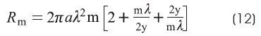
The Hodgkin and Rushton's article¹ was very important for understanding the passive properties of the axon^6,13. Theoretical equations which reproduce the response of the nerve fiber to a stimulus current were derived from their results. According to Hodgkin and Rushton¹ the most important reason for conducting an analysis of the passive properties of a nerve fiber is that such analysis is necessary for an understanding of the more complicated electrical changes which make up the nervous impulse itself⁶. The passive behavior of the fiber can be determined by four electrical constants: (1) The electrical resistance of the fluid outside the nerve fiber, (2) The electrical resistance of the axoplasm, (3) The electrical capacity of the surface membrane, and (4) the electrical resistance of the surface membrane^1,4,7,8. The external resistance can be calculated from the volume and conductivity of the fluid bathing the nerve¹. The cell interior appears to have a resistivity two or three times as great as that of the external fluid (50 Ωcm, Rall²) and the surface membrane appears to have a capacity of about 1 μF/cm² (0.7-1.3 μF/cm², Genter et al⁴). Due to the inherent difficulties to measure the resistance of the membrane, Hodgkin and Rushton have proposed to combine their experimental data with a mathematical model (equation 12) in order to get such measurement¹.

In order to evaluate the electrical constants, Hodgkin and Rushton¹ used the following methods: (1) The extent of the spread of potential in the extrapolar region (the extrapolar region is the axonal membrane outside of the stimulation electrodes; the electrotonic potential is measured here at different distances from the current source), (2) The rate of rise in potential in the extrapolar region, (3) The ratio of the applied current to the voltage recorded between cathode or anode and a distant extrapolar point, and (4) The voltage gradient at the midway point between two distant electrodes (interpolar region).

The extrapolar region method is used to determine the time constant (τ_m) and the space constant (λ). The interpolar region method allows the measurement of input resistance equivalent (y) and the calculation of the parallel resistance of the axis cylinder and external fluid (m), the specific resistivity of the axoplasm (R_i), and the specific resistance of the membrane (R_m).

Hodgkin and Rushton derived all the equations necessary for the adequate reproduction of all of their experiments^1,6.

Cable theory is useful in coordinating a wide range of experiments. The transient solution of the cable equation for an infinite cable at X = 0 above is extremely useful because it describes the charging curve at the site of current injection, the usual site of potential measurement¹³. It would also be useful, however, to know what the transient change in membrane potential would be at different sites from that of current injection^1,13. The current flows longitudinally along the axon, and as it moves away from the electrode, some of it is lost on account of ion movements through the membrane^1,6,13.

The equivalent circuit is a series of resistive elements, r_m and r_i, connected in a chain.^1,6,7,13. The membrane resistance, r_m, represents the resistance across the cylinder wall; the longitudinal resistance, r_i, representthe internal resistance along the axoplasm (Figure 1A). The distance the potential spreads along the axon depends on the resistance of the cell membrane relative to that of the axoplasm^1,6,7,13,15. Because nerves in a recording chamber are normally bathed in a large volume of fluid, the extracellular longitudinal resistance along the cylinders is represented as zero. In Hodgkin and Rushton, r_m /r_i > 0.

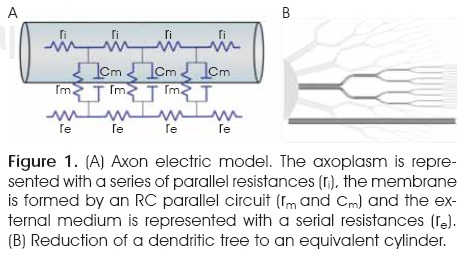
B. Dendritic tree model

Shapes of dendrites are not only complex, but also highly variable from one neuronal type to another. This diverse shape of dendritic trees contributes to differential processing of inputs by different classes of neurons. Rall's theoretical model enables the simplification of the complex structure of a dendritic tree. The principal objective was to harness the equations derived from experiments in the axon. One of Rall's major contributions was to show how a complicated tree structure such as this could be reduced to a single equivalent cable. His aim was to provide a method for simplifying the complex geometry of a branching dendritic tree, while preserving its electrical properties. The method he used was a recursive calculation for the steady-state input conductance of a finite length of a cylindrical dendrite which terminates with further branching. Each dendrite length was terminated by a conductance which constituted the input conductance of the subsequent branching. Repeated substitutions for the input conductance at each branch point led to a compact expression for the input conductance of a dendritic trunk. Rall makes the important observation that the diameter of dendritic branches obey the 3/2 power rule. Then, for passive dendritic trees fulfilling certain symmetry conditions, the reduction to an equivalent cable can be justified on theoretical grounds^12,16,17.

The development of a mathematical model of dendritic neurons began due to the need to combine three different strands of knowledge into a coherent theory: (1) The anatomical concept of the neuron, together with the anatomical understanding that extensive dendritic branching is characteristic of many important neuron types, (2) The theoretical development of the nerve membrane models, (3) The detailed body of quantitative electrophysiological information that has been obtained from individual neurons by means of intracellular and extracellular microelectrodes¹⁵.

In dendritic neurons, the effective R_m can vary, from valuesoflessthan 1,000 Ωcm² to more than 1,000,000 Ωcm² in different neurons^18-23. Traditionally, the value of Ri has been believed to be in the range of approximately 50 - 100 Ωcm based on muscle cells and the squid axon. In mammalian neurons, estimations now tend toward a value of 200 Ωcm^18,22-26.

The Hodgkin and Rushton's model and that at Rall may be used as long as certain assumptions are taken into account. First of all, the geometric and passive electric properties of an axon and neuron with dendritic trees must be idealized to produce a formal theoretical model that is suitable for mathematical treatment¹⁸. The necessary assumptions and definitions for the two simulators are listed in Table 2.

 

DEVELOPMENT OF THE SIMULATOR

Microsoft Visual Basic^® version 5.0 for IBM PC or compatible was used to create the simulator. The minimal requirements for the software are: Pentium III, 350 MHz or higher, Windows 98 or higher, SuperVGA Monitor with a resolution of 1,024 x 768 pixels or higher, and at least 7 MB of free space on the hard drive.

The development of the simulators is based on cable theory. In the simulators x is distance along the axon in cm, t is time in seconds and i₁ is the current in amperes flowing through the external fluid.

The cable equation is:

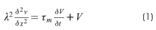
Where:

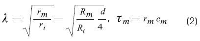
λ, has distance dimensions and is known as the space constant. It determines the tendency for current to flow along the cable. The space constant depends not only on the internal membrane resistance, but also on the diameter of the axon.

τ_m is the membrane time constant.

In Hodgkin and Rushton's work:

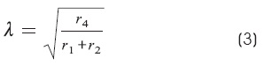
Where:

r₁ is the resistance per length of the external fluid
r₂ is the resistance per length of the axis cylinder
r₄ is the resistance per length of the surface membrane in the axon

The cable equation can be put into its most general and useful form by normalizing the length constant (space constant) and the time constant. Where X = x/λ and T = t/τ_m, the equation becomes^3,6,9:

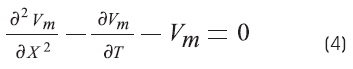
Where X and T are dimensionless

 

A. HR2 simulator

The solution of the cable equation for infinite cable for a step current at X = 0 is^1,6:

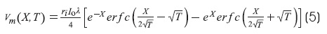
This equation corresponds to boundary conditions of infinite cable.

Where erfc(x) = complementary error function and erf(x) = error function^1,6:

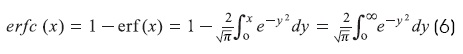
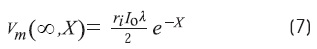
Where erf(0) = 0, erf(∞) = 1, and erf(-x) = -erf(x) The steady-state solution (T →∞) is:

The measurement of «y» (Ω)

The constant y (R - input equivalent) is given by the rate of the steady voltage at the cathode to the applied current, hence:

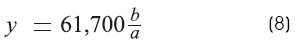
Where

a is the recorded voltage (x = 0).
b is the stimulus voltage.
61,700 Ω is the resistance of the external electrode.

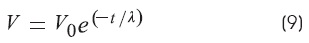
The length constant (λ) is the reciprocal of the rate of decay voltage along the cable distance:

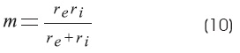
The measurement of «m» (Ω/cm):

m has been defined as the parallel resistance of core and external fluid. It was determined by measuring the voltage gradient midway between two distant electrodes and dividing the gradient by the current through the nerve (interpolar region):

R_i is the specific resistivity of the axoplasm:

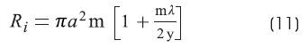
Where:

α is the cylinder's radius in cm.

R_m is the specific resistance of the membrane:

The program follows Hodgkin and Rushton's experimental procedure:

• The user inputs the values (in this version this step can be omitted as the values are randomly generated by the program).

• The extrapolar region is simulated: spread of potential along a lobster axon, recorded with a surface electrode. In this simulation τ_m at X = 0 is calculated.

• The plot voltage - vs- distance is showed and λ is calculated.

• The intrapolar region is simulated: This procedure measures the voltage gradient in the region midway between two distant electrodes. The program calculates the input resistance equivalent (y), m, R_m and R_i.

 

B. Rall1 simulator

In Rall's equivalent cylinder morphological to electrical transformation, neuronal arborizations are reduced to single unbranched core conductors. The conventional assumption that such an «equivalent» reconstructs the electrical properties of the dendritic tree is shown in the Table 2.

The model was based on a set of carefully chosen symmetries that simultaneously abstracted the neuron and simplified the mathematics (Figure 1B).

The simulator Rall1 uses the general solution of the cable equation (equation 4) in terms of hyperbolic function. The cable equivalent has different end terminations, each of which has a different boundary condition.

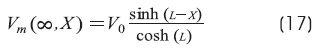
The steady-state solution of the cable equation for a finite-length cable is^13,18,24:

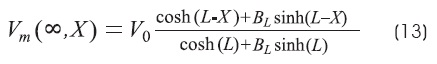
B_L is the boundary condition for different end terminations:

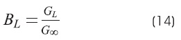
Where:

G_L is the conductance of the terminal membrane.

G_∞ is the conductance of semi-infinite cable.

For the two types of terminations, G_L will be zero for the sealed end and infinite for the open end. We will consider three cases:

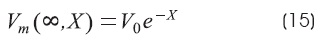
Infinite cable extension: B_L = 1 (that is G_L = G_∞)

Cable with sealed-end condition: B_L = 0 (G_L<<G_∞)

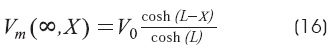
Cable with open-end condition: B_L = ∞ (G_L >> G_∞)

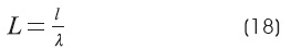
The length of cylinder in terms of λ (dimensionless electrotonic length) is:

Dendritic to soma conductance ratio.

The rate of combined dendritic input conductance to the soma membrane conductance is:

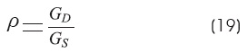
Where:

G_D is the dendritic input conductance.

G_S is the soma membrane conductance.

 

RESULTS

Program installation

The simulator is installed through the «setup» file, which guides the user step by step to correctly install the software. By using the program HR2, the students may select a variety of experimental conditions. The simulated experimental setup consists of an oscilloscope, shown at the right side of the windows interface, and the nerve preparation shown to the left (Figures 2 A and B).

 

A. HR2 simulator: Interface and use

A Hodgkin and Rushton experimentiscarried out as follows:

Input windows interface: From top to bottom, the interface shows the values of the fiber diameter (60 to 87 μm), external resistance per unit length (r_i) (150 to 250 Ω/cm), internal resistance per unit length (r_e) (130 to 250 Ωcm), membrane resistance per unit length (r_m) (350 to 1,500 Ωcm), membrane capacitance (c_m) (400 to 3,240 nF/cm) and stimulus strength (2 to 9 μA)^1,6.

First step: The user selects the corresponding values for the simulation. A scrollbar is used to introduce each of the values.

Recording windows interface: The program HR2 version 2.0 has two options; extracellular or intracellular recording. This interface shows, on the left hand side, the schematic preparation of the axon. The scrollbar is used to move the recording electrode along the nerve. The button «STIMULUS» is used to apply the stimulus current. The right side shows the oscilloscope.

At the bottom left there are 4 buttons: «LENGTH CONSTANT» (which sends the user to the interface to calculate λ), «R-input EQUIVALENT (y)» (which sends the user to the interface to calculate (y)), «INTERPOLAR REGION» and «INTRACELLULAR RECORD» (which sends the user to the recording corresponding windows). At the bottom right, there aretwobuttons: «reset» (clear the oscilloscope), and «TIME CONSTANT» (calculate the τ_m at X = 0 μm) (Figure 2A).

In this step, the student records along a lobster axon. The τ_m is calculated at X = 0 (Figure 2A). A rectangular current pulse is applied at 0 mm, producing an electrotonic potential. With increasing distance from the site of current injection, the rise time of the potential change is slowed and the plateau attenuated (Figure 3A)¹. At any time, the user can change parameter values and observe the consequences.

Next step, the user presses the button «LENGTH CONSTANT». The plot windows interface shows two boxes for the plotting results (Figure 2E). The bottom screen contains two buttons: «GO» and «R-input EQUIVALENT (y)». The button «GO» is used to show the steady state membrane potential as a function of distance in the axon in response to current injection at one end (X = 0 μm). The λ is the reciprocal of the rate of voltage decay along the cable distance. The user obtains the λ values.

The R-input EQUIVALENT interface shows the schematic preparation of the measurement of the voltage in the stimulus electrode. On the right side, there are three boxes showing the recorder voltage (X = 0 μm), stimulus voltage and input resistance equivalent respectively. In this step, the user presses the button «STIMULUS» to calculate these values (Figure 2C). Next step, the user presses the button «INTERPOLAR REGION».

The interpolar region interface presents, on the left side, the schematic preparation and in the right side the oscilloscope (Figure 2D). These windows presents the button «Reset» to clean the oscilloscope and «GRAPHIC» to go to the corresponding plot interface. In this step, constant «m» can be obtained from a measurement of the voltage gradient in the interpolar region at a large distance from either stimulus electrode (Figure 3B). The user presses the button «Stimulus» and moves the scrollbar to simulate the movement of the electrode register at different points along the length of the axon.

There are three boxes in the window: The first is the distance in which the register was made, the second is the maximum voltage reached and the third is the resistance obtained with experimental data.

The «GRAPHIC» button takes us to the interface in which appears a chart for calculating resistance in the experiment versus the distance in which the register was made (Figure 2F). The user interface located from top to bottom on the right side, has three boxes showing the m, R_i and R_m respectively. On the bottom right side there are two buttons: «EXTRAPOLED REGION» and «GENERAL RESULT».

At this stage, if we press the «GO» button, it creates a chart showing a linear process. The «m» parameter is the slope (Figure 2F). From λ, «y» and «m» parameters the corresponding R_i y R_m values (equations 11 and 12) can be calculated.

Finally, the final results are made to appear by pressing the «GENERAL RESULT» button. From top to bottom, the resistivity of the axoplasm (R_i), specific membrane resistance (R_m), the diameter of the axon, «y» parameter, «m» parameter, length constant λ and membrane time constant τ_m are shown.

As an example: (1) enter the following values: diameter = 65 μm, r_e = 160 and r_i = 180 (Ω/cm), r_m = 850 Ωcm, c_m = 1,000 nF/cm and stimulus = 4 μA. The Figure 3A shows the registered voltage and how it decreases as the register electrode moves away from the stimulus point.

The results of this experiment are R_i = 59.72 Ωcm, R_m = 1,735 Ωcm², diameter 65 μm, input resistance = 59.52 kΩ, λ = 1.58 mm and τ_m = 1.73 ms. These values are consistent with those obtained by Hodgkin and Rushton in Table 2 of their paper¹.

Another example: (2) go directly to the experiment. This condition emulates actual conditions because usually the researcher is unaware of the axon resistance and capacitance values. The goal is to calculate them from the experimental process. In this case the results were: R_i = 73.12 Ωcm, R_m = 2,089 Ωcm², diameter 70 μm, input resistance = 65.2 kΩ, λ = 1.62 mm and τ_m = 2.5 ms. Again it can be observed that these values are consistent with those obtained by Hodgkin and Rushton in their experiment¹.

Each user interface has a menu in the upper left corner of the screen in which the user can access a help box to display a definition of each of the concepts involved in the experiment, the corresponding equations and their equivalence with the actual nomenclature (Table 1).

 

B. Rall1 simulator: Interface and use

This program simulates voltage response to a stimulus of subumbral current in an isopotential cell, in dendrites and neurons with dendrites^13,18,24. Use of this program allows the student to become familiar with subjects which, because of the mathematics they entail, are not generally approached and are rarely understood. The synaptic integration in the neurons depends to a certain extent on the passive properties. Synaptic integration is fundamental to neural communication and thus fundamental to the function of the nervous system.

The simulator is installed through the «setup» file which guides the user step by step to correctly install the software. A file named Rall1.exe is opened to execute the program. The Start option of Microsoft Windows gives the option to open a window with the main menu which then gives the option of selecting from three modules: (1) isopotential cell, (2) equivalent cylinder models, (3) soma model + equivalent cylinder.

The isopotential cell module shows the case of ideal neurons without dendrites (as could be the case with some ganglionar neurons or bipolar cells). This case considers spherical cells in which the membrane potential is uniform at all points of the sphere. R_m is constant and independent from voltage. The electrical model in these cells is an RC circuit in parallel.

 

1B. «Isopotential Cell» module: User interface

Figure 4A shows the user interface for this module. On the upper left hand corner there are two boxes in which to input data for membrane potential and applied current amplitude (nA). Below, there is a diagram of the cell in which arrows indicate how current is distributed in a uniform way in every direction within the cell. The right half of the screen shows two boxes that represent the oscilloscope. The current pulses of the stimulus are displayed in the upper box and the charge curves that correspond to these stimuli are shown in the lower box. Underneath this box there are two buttons: «Start» which executes the simulation and «Erase» which clears the boxes. Bellow that there is the button «Back» which leads to the main menu (Figure 4D) and «Exit» to quit the program. A help menu appears in the upper part of the window.

Use: the student inputs the value of the membrane potential and the amplitude of the stimulus. For instance: a value of -80 mv was given and the stimulus amplitude values as follows: 2, -2, 3, -3, 4, -4 (nA). The curves of positive and negative charges are shown in relation to the polarity of the stimulus pulse. The simulation corresponds to Figure 4. 5 in Johnston and Wu¹³. The appropriate moment to calculate the time constant of the cell (τ_m), deduce the differential equation in relation to the electric model and to solve the equation is considered. In the «Help» menu one can find the corresponding mathematical information^11-13.

 

2B. «Equivalent cylinder model» module: User interface

Figure 4B shows the interface window. The left half presents a diagram with circles that represent the channels of the membrane (these are not the usual channels which depend on voltage). A sliding bar appears next to it that allows us modify the electronic longitude value (L) with said values being shown in a box underneath. Further below there are three equivalent cylinders: the first is long and considered infinite, the next is short with open ends and the last is short with sealed ends. A corresponding button is found next to each cylinder to run the simulation in each case. On the right side of the window, a box shows the voltage decay in relation to distance. Below there are two buttons: «Erase» and «Back».

Use: As was the case of the first interface, the student can move the sliding bar to input a value of electronic longitude (L). In the «Help» menu one can find a definition of L¹⁸. This is useful to help the student understand the difference between physical longitude and electronic longitude^16,19,22,23. Later one can activate the button for each of the equivalent cylinder conditions and the corresponding voltage decay is shown. As an example: an electronic longitude of 1.7 was inputted and simulations for each condition were run. The upper stroke represents the short cylinder with sealed ends, the middle stroke represents the voltage decay in the long infinite cylinder and the lower stroke denotes the short open ended cylinder. Figure 4B shows the distributions of electronic potential along unbranched cylinders for different terminal boundary conditions and different lengths. It can be observed that the decay voltage in a short open cylinder reaches zero, and the infinite cylinder also tends to zero but over a longer distance, while with the sealed cylinder the voltage remains high. This simulation is similar to Figure 4.15 in Johnston y Wu¹³ and Figure 3 in Rall¹⁶.

 

3B. «Soma model + equivalent cylinder» module: User interface

This module allows for the use of p as proposed by Rall, to determine the predominance of the dendritic tree in the neuron. To a higher value of p the neuron presents a more abundant dendritic tree. A value of zero corresponds to an isopotential neuron and an infinite value corresponds to a cylinder.

Figure 4C shows the user interface. On the left side of the window one can find the oscilloscope, where the charge curves generated in response to a current stimulus are shown²⁵. On the right side, there are three diagrams representing the simulation conditions. The lower diagram corresponds to an isopotential cell (p = 0), while the diagram above corresponds to a cylinder (the soma electrical characteristics are such that it can be merged to the dendritic tree and be considered whole as a cylinder (p = infinite))^18,19. The diagram above the previous corresponds to a neuron with dendrites, in which the value of p can be adjusted and thus the curve charge of neurons with different dendritic abundance can be simulated. An illustration showing different values of p is shown in Figure 4D, on the left side^13,18.

 

DISCUSSION

Physiology, Biophysics or Neuroscience college courses have little to do with neuronal passive properties. Text books such as The physiology of excitable cells by Aidley²⁶; Biofísica y fisiología celular by Latorre et al²⁷; From neuron to brain by Nicholls et al¹⁵ and Principles of neural science by Kandel et al²⁸ touch on this theme no more than summarily.

There is no specific simulation software dealing with the passive properties of the axon and the dendritic tree through analytical solutions using cable theory that can be used as a teaching tool.

This simulator reproduces Hodgkin and Rushton's experiments virtually using cable equations and their analytical solutions. Up to date, there is no other simulator that reproduces these experiments. The cable model has been widely used in order to determine the passive properties of several neurons and with enough symmetry to reduce it to an electrically equivalent cylinder^19-21,29. «The exponential peeling method» proposed by Rall¹⁸ allows us calculate the passive parameters from experimental data using an analytical treatment from Rall's cable theory¹⁸.

While Rall's model is based on the assumption of an homogeneous R_m other models have been developedconsideringa heterogeneous membrane (with the somatic resistance lower than the dendritic resistance) based on an equivalent cylinder^29-31.

The strength of the equivalent cylinder concept has been proved in Ohme and Schierwagen's³² work, where they show several dendritic trees reduced to different equivalent cylinders with added active properties. In those cases where Rall's branching rule no longer functions, it can be reduced to a non uniform diameter cable.

Rall's paper³³ is one of the most significant landmarks in the modern era of computational neuroscience. Rall introduced the compartmental modeling method, which, in principle, allows the computation of voltage and current spread in no idealized, and hence, biologically realistic trees, with any specified voltage and with non-linear active properties³³.

Programs such as Genesis or Neuron work effectively to simulate specific neurons and provide corresponding anatomical data and electrophysiologic studies³⁴. These programs have interactive computer tutorials that include concepts in neuroscience and neuronal modeling. For example the developers of GENESIS have published «The book of GENESIS», including an outline of cable theory aimed at the development of passive compartmental models. However, they omit Rall's equivalent cylinder theory and Hodgkin and Rushton's¹ classic experiment simulations. From the point of view of the authors of this article, these experiments are fundamental to understanding cable theory principles. The simulations of virtual experiments, such as the interactive programs described in this paper, introduce students to this topic.

We recommend students to conduct the simulations in the classroom, and to explain and present the corresponding mathematical equations in every case as part of an intuitive approach. Additionally, the compartmental models from GENESIS³⁴ or Neuron³⁵ can be used to complement the topic.

It is important to mention that concepts involved in compartmental models originate in cable theory. Each compartment is represented by a differential equation. In general, cable theory and compart-mental modeling provide a foundation for predicting the propagation of electrical signals in the dendrites and axons of neurons^36,37.

For the HR2 simulator we recommend the user to follow Hodgkin and Rushton's experiment stages. It is desirable but not necessary to read these researchers' papers and simulate every part they describe.

Similarly, for the Rall1 simulator it is recommended, that the simulations begin in the order in which they appear in the main menu. The simulator design has been developed as a powerful didactic tool to be used alongside relevant and appropriate texts, such as Chapter 4 from «Foundations of cellular neurophysiology» by Johnston and Wu¹³.

These simulators have been used for the last three years in the Biophysics module in the Biology School at the Benemérita Universidad Autónoma de Puebla (BUAP), and have been constantly improved on based on the (unpublished) results obtained from a survey measuring student satisfaction. In general, feedback has been sought from students in terms of the usefulness of the software in two dimensions: (1) usability of the simulator, and (2) its facilitation of learning. In both cases, these elements are evaluated through closed answers (very adequate, adequate, slightly adequate and in no way adequate) and (very good, good, average, unsatisfactory) respectively.

Some of the applied questions are:

Did you learn how to obtain space constant?

Did you learn how to obtain time constant?

Can you predict what will happen to time constant when r_m changes?

Did you identify the effect that produces the changes in the variables r_m , r_i, r_e y C_m , in the passive properties of the axon?

Finally, the program explores the students' perception of the utility of mathematical and computational tools in their professional formation.

The students consider that simulators are easy to use. All students changed their perception of neuroscience and discovered a new way of applying mathematics. The 96.5% now accept as valid the use of mathematics in their profession and are willing to learn more about this application, 30% of students indicated that the discipline they were inclined to study had changed from another discipline to neurosciences, and 3.5% of students had not adapted to the use of simulators.

In conclusion, these results show that using simulators as a didactic tool in the teaching of these apparently difficult topics may change student perception and stimulate their interest to study and use simulators.

 

ACKNOWLEDGEMENTS

We thank PIFI 2011 for the support given to this publication.

 

REFERENCES

1. Hodgkin AL, Rushton WAH. The electrical constants of a crustacean nerve fibre. Proc Roy Soc Lond B 1946; 133(873): 444-479.         [ Links ]

2. Rall W. Branching dendritic trees and motoneuron membrane resistivity. Experimental Neurology 1959; 1: 491-527.         [ Links ]

3. Koch C. Biophysics of computation. Oxford University Press, New York, 1999; pp. 25-48.         [ Links ]

4. Clark JW, Plonsey R. The extracellular potential fied of the single active nerve fiber in a volume conductor. Biophys J 1968; 8: 842-864.         [ Links ]

5. Tuckwell HC. Introduction of theoretical neurobiology. Vol 1: Linear cable theory and dendritic structure. Cambridge University Press, 1988; pp. 124-282.         [ Links ]

6. Jack JJB, Noble D, Tsien RW. Electric current flow in excitable cells. Clarendon Press, Oxford, 1975; pp. 25-82.         [ Links ]

7. Davis L Jr., Lorente de No R. Contribution to the mathematical theory of the electrotonus. Stud Rockefeller Inst M Res, 1947;131: 442-496.         [ Links ]

8. Clark JW, Plonsey R. A mathematical evaluation of the core conductor model. Biophys J 1966; 6: 95-112.         [ Links ]

9. Kootsey JM. The steady-state finite cable: numerical method for non-linear membrane. J Theor Biol 197; 64: 413-420.         [ Links ]

10. Arthurs AM, Arthurs WM. Pointwise bounds for the solution of a nonlinear problem in cell membrane theory. Bull Math Biol 1983; 45: 155-168.         [ Links ]

11. Rall W. Cable theory for dendritic neurons. In: Methods in neuronal modeling. Koch C. and Segev I, editors. MIT Press, Cambridge, 1989; pp. 9-12.         [ Links ]

12. Segev I, Rinzel, J, Sheperd, GM. The theoretical foundation of dendritic function. The MIT Press, Cambridge, Massachusetts, 1995.         [ Links ]

13. Johnston D, Miao-Sin Wu S. Foundations of cellular neurophysiology. The MIT Press, Cambridge, Massachusetts, 1995; pp. 55-120.         [ Links ]

14. Genter LJ, Stuart GJ, Clements JD. Direct measurement of specific membrane capacitance in neurons. Biophys J 2000; 79: 314-320.         [ Links ]

15. Nicholls JG, Martin RA, Wallace BG, Fuchs PA. From neuron to brain. Sunderland, Massachusetts, 2001; pp. 113-132.         [ Links ]

16. Rall W. Membrane time constant of motoneurons. Science, 1957; 126:454-493.         [ Links ]

17. Schierwagen AK. A non-uniform equivalent cable model of membrane voltage changes in a passive dendritic tree. J Theor Biol 1989; 141: 159-179.         [ Links ]

18. Rall W. Core conductor theory and cable properties of neurons. In Handbook of physiology. Sec. 1, The nervous system, vol. 1. Bethesda, MD: Am Physiol Soc 1977; pp.39-97.         [ Links ]

19. Brown TH, Perkel DH, Norris JC, Peacock JH. Electrotonic structure and specific membrane properties of mouse dorsal root ganglion neurons. J Neurophysiol 1981; 45(1): 1-15.         [ Links ]

20. Stafstrom CE, Schwindt PC, Crill WE. Cable properties of layer V neurons from cat sensorimotor cortex in vitro. J Neurophysiol 1984; 52(2): 278-289.         [ Links ]

21. Bargas J, Galarraga E, Aceves J. Electrotonic properties of neostriatal neurons are modulated by extracellular potassium. Exp Brain Res 1988; 72: 390-398.         [ Links ]

22. Iansek R, Redman SJ. An analysis of the cable properties of spinal motoneurones using a brief intracellular current pulse. J Physiol 1973; 234: 613-636.         [ Links ]

23. Burke RE, Fyffe REW, Moschovakis AK. Electrotonic architecture of cat gamma motoneurons. J Neurophysiol 1994, 72: 2302-2316.         [ Links ]

24. Rall W. Electrophysiology of a dendritic neuron model. Biophys J 1962; 2: 145-167.         [ Links ]

25. Rall W. Membrane potential transients and membrane time constant of motoneurons. Exptl Neurol 1960; 2: 503-532.         [ Links ]

26. Aidley JD. The physiology of excitable cells. 4th edition, Cambridge University Press. New York, USA. 1998.         [ Links ]

27. Latorre R, López-Barneo J, Bezanilla F, Llinás R. Biofísica y fisiología celular. Universidad de Sevilla, Santiago de Chile. 1986.         [ Links ]

28. Kandel ER, Schwartz JH, Jessell TM. Principles of neural science. 4th edition, McGraw Hill, New York, 2000.         [ Links ]

29. Reyes A, Galarraga E, Flores-Hernández J, Tapia D, Bargas J. Passive properties of neostriatal neurons during potassium conductance blockade. Exp Brain Res, 1998; 120(1): 70-84.         [ Links ]

30. Kawato M. Cable properties of a neuron model with non-uniform membrane resistivity. J Theor Biol 1984; 111: 149–169.         [ Links ]

31. Holmes WR, Rall W. Electrotonic length estimates in neurons with dendritic tapering or somatic shunt. J Neurophysiol 1992; 68(4): 1421-1437.         [ Links ]

32. Ohme M, Schierwagen A. An equivalent cable model for neuronal trees with active membrane. Biol Cybern 1998; 78: 227-243.         [ Links ]

33. Rall W. Theoretical significance of dendritic trees for neuronal input-output relations. In Neural theory and modeling, ed. RF Reiss, Palo Alto, Stanford University Press, 1964.         [ Links ]

34. Bower JM, Beeman D. The book of GENESIS. 2nd edition, Springer and Telos, New York, 1998.         [ Links ]

35. Carnevale NT, Hines ML. The NEURON book. Cambridge University Press, 2005.         [ Links ]

36. Hines ML. Efficient computation of branched nerve equations. Int J Biomed Comput 1984; 15: 69-76.         [ Links ]

37. Cannon RC, O'Donnell C, Nolan MF. Stochastic ion channel gating in dendritic neurons: Morphology dependence and probabilistic synaptic activation of dendritic spikes. Comp Biol 2010; 6(8): 1-18.         [ Links ]