


 nueva página del texto (beta)
 Inglés (pdf)
 Artículo en XML
 Referencias del artículo
 Enviar artículo por email
 Citado por SciELO
  Similares en
SciELO
Similares en
SciELO 
 Permalink
1. Introduction
It is well-known that the organization of squall lines (SLs) is strongly dependent on the environmental vertical wind-shear throughout the low and mid-troposphere (Thorpe et al., 1982; Barnes and Sieckman, 1984; Bluestein and Jain, 1985; Rotunno et al., 1988, hereafter RKW88; Fovell and Ogura, 1989; Alfaro, 2017). The magnitude of the shear can affect a SLs maintenance (Coniglio et al., 2007; Alfaro and Coniglio, 2018), its precipitation rate (Rotunno et al., 1990; Weisman and Rotunno, 2004, hereafter WR04; Bryan et al., 2006; Alfaro, 2017), mesoscale circulations within the stratiform region (Lafore and Moncrieff, 1989; Weisman, 1992; Parker and Johnson, 2004a), and the intensity of surface wind speeds (Weisman, 1993; Bryan et al., 2006; Cohen et al., 2007). But consensus about the physical mechanisms governing the interactions between SLs and the low-to-mid-tropospheric shear is lacking within the community of mesoscale meteorologists, as reflected by decades of vigorous scientific debate continuing to this date (e.g. WR04; Stensrud et al., 2005; Bryan et al., 2012; Coniglio et al., 2012; Alfaro, 2017). Thus, further research on storm-shear interactions is warranted, especially because better understanding of such processes might lead to improved forecasts (e.g. Coniglio et al., 2007; Alfaro and Coniglio, 2018) and parameterizations (e.g. Dai, 2006; Moncrieff, 2010).
The leading paradigm for explaining how the low-to-mid-tropospheric shear affects SLs with well-defined cold pools (e.g. Bryan et al., 2005; Engerer et al., 2008; Bryan and Parker, 2010; Provod et al., 2016) is RKW88’s theory of vorticity-balance (hereafter RKW theory). RKW theory contends that the orientation and intensity of the deep convective updraft, a fundamental structural element of SLs, is primarily determined by the amount of baroclinically generated vorticity at the edge of the cold pool relative to the inflowing environmental vorticity due to the shear. Specifically, RKW88 refer to the horizontal vorticity equation to argue that the shear’s vorticity, which favors downshear updraft tilting (Asai, 1964), can counter the cold pool’s tendency to “sweep” parcels over the denser air when both vorticity sources have opposite signs and similar magnitude. Per RKW theory, a SL’s updraft leans downshear (upshear) if the shear’s vorticity inflow is greater (less) than the baroclinically generated vorticity, with updraft verticality depending directly on the degree of vorticity-balance. And given that slanted updrafts tend to be weaker than vertically oriented ones (Asai, 1964; Lilly, 1979; Parker, 2010), RKW theory also ostensibly explains the intensity and depth of ascending motions.
To evaluate their theory, RKW88 derived a quantitative diagnostic from the vorticity equation in density currents, where the denser fluid represents a SL’s cold pool. They found that in steady systems with strictly vertical updrafts, referred to as “optimal” (Bryan and Rotunno, 2014, hereafter BR14), the density current’s theoretical propagation speed (c) (Benjamin, 1968), which measures the rate of baroclinic vorticity generation, must equal the change in wind speed within the shear-layer (∆U), which measures the shear’s vorticity inflow. This result led to the conclusion that upshear (downshear) leaning updrafts arise when c is greater (less) than ∆U, a matter substantiated in RKW88 by density current simulations. Thereafter c/∆U has been the focus of many numerical studies which find that simulated density currents (e.g. WR04; BR14) and SLs (e.g. Weisman et al., 1988; Rotunno et al., 1990; Weisman, 1992; WR04; Bryan et al., 2006) behave as predicted by RKW theory, leading WR04 to state that cold-pool-shear relationships “represent the most fundamental internal control on squall-line structure and evolution”.
For all its apparent success, there is ample evidence that RKW theory is not as restrictive on the structure of SLs (e.g. Parker and Johnson, 2004b) and density currents as suggested by the studies mentioned above. For instance, Alfaro (2017) showed that ∆U affects the intensity of SL’s primarily through its impact on layer-lifting convective instability, rather than vorticity-balance effects, perhaps explaining the lack of robust observational evidence for RKW theory (Evans and Doswell, 2001; Gale et al., 2002; Stensrud et al., 2005; Coniglio et al., 2012). More relevant to this study is the fact that RKW theory does not provide a strict criterion for determining the depth over which ∆U should be computed. This is important because SLs organize in a variety of kinematic environments (Evans and Doswell, 2001; Gale et al., 2002; Cohen et al., 2007; Coniglio et al., 2007; Coniglio et al., 2012), and these systems are known to be sensitive to the shear-layer depth, for a given c/∆U (e.g. WR04). Furthermore, BR14 found that density currents with c ≈ ∆U can develop shallow, tilted updrafts, both in the downshear and upshear directions, depending on the depth of the shear-layer; conversely, highly vorticity-unbalanced flows can develop vertical updrafts if a suitable shear-layer depth is chosen (see BR14, Fig. 18). These findings challenge the commonly held notion that c/∆U provides a strong constraint on an updraft’s orientation and depth, both in SLs and density currents.
The objective of this research is to develop a theory of storm-shear interactions that accounts for the impacts of the shear profile, especially the shear-layer depth, on an updraft’s structure. For simplicity, only adiabatic density current simulations will be considered, as described in subsection 2.1. Subsection 2.2 reviews the theoretical foundations of RKW theory, where we argue that c/∆U is not a robust measure of vorticity-balance for non-optimal flows, being better suited for measuring the strength of system-relative wind velocities aloft, whose relevance was noted by Thorpe et al. (1982). Per this interpretation, c/∆U is pertinent to the updraft’s structure aloft, so we seek a framework for diagnosing the updraft’s structure throughout low-to-mid-levels. Motivated by BR14’s results showing that the flow-force balance constraint of Benjamin (1968) is a necessary condition for optimal density currents, subsection 2.3 explores the application of momentum-balance concepts for defining a metric (MB) to diagnose the updraft’s orientation at low and mid-levels. In order to validate our interpretation of c/∆U and the momentum-balance framework, 2D adiabatic density currents are simulated following the methodology of BR14, as described in section 3. Section 4 analyzes the results by contrasting the diagnostic skill of MB to that of c/∆U. Results are discussed in Section 5, while a summary and future work around applications to SLs are presented in Section 6.
2. Vorticity-balance and momentum-balance in density currents
2.1 Adiabatic, inviscid, incompressible, and steady density currents
This subsection considers density currents, as those depicted in Figure 1. Density currents are frequently used to study storm-shear interactions (RKW88; Liu and Moncrieff, 1996; WR04; Alfaro, 2017), as they have many features in common with cold pools (Charba, 1974; Wakimoto, 1982), while being much simpler than SLs.
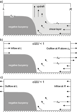
Fig. 1 Schematic depiction of density currents. The dark-gray area corresponds to the denser fluid, while arrows indicate the flow at lateral boundaries and near the density current’s edge. The flow in a) has a vertical updraft, with static air outside the region in light-gray. Cases in b) and c) have c/∆U < 1 and c/∆U > 1, respectively.
The density current analysis is based on the 2D, incompressible, adiabatic, and inviscid Boussinesq equations in a neutrally stratified fluid:
where u and w are the horizontal and vertical components of the wind velocity, respectively, ρ 0 is (constant) density, p is pressure, b = -g ρ'/ρ 0 is buoyancy, and g is the constant of gravitational acceleration. The naught symbol indicates constants that characterize the light fluid, while primed variables are perturbations with respect to the environment, i.e. the flow at R in Figure 1a.
To delimit the problem, consider a steady density current (Fig. 1; the frame of reference is such that air is static within the density current). The fluid is infinitely deep, with open lateral boundaries and a rigid, flat, and free slip lower boundary. Pressure is assumed to be constant at the upper boundary and the flow at both lateral boundaries is hydrostatically balanced, i.e. the rhs of (2) is equal to zero. With these assumptions, the conservation of Bernoulli energy can be applied to the inflow streamline from R to the density current edge to determine the environmental surface wind speed (Xu, 1992):
where the first subscript specifies lateral boundaries L or R (Fig. 1) and the second subscript specifies height (z). Applying hydrostatic balance, while considering ρ' L = 0 for z > z dc , where z dc is the density current depth, (5) can be expressed as
Note that c in (6) equals the density current’s theoretical propagation speed, as defined by RKW88, and that u R,0 = c is a consequence of the assumptions made. In addition, mass conservation in an infinitely deep fluid requires u L ≈ u R some distance above z max = max(z sh , z dc ) < ∞, where z sh is the environmental shear-layer height, which is consistent with density current simulations analyzed in RKW88 and BR14. In other words, if one considers a fluid of depth z* with a given u R profile, then mass conservation requires that the inflow/outflow at L satisfies ∫0 z* u L dz / ∫0 z* u R dz = 1; this condition is satisfied in the limit z* → ∞ when winds aloft at L equal winds aloft at R (this is a consequence of the intuitive fact that winds above z max dominate the mass flux at lateral boundaries as z* → ∞). These are the working assumptions for all subsequent analyses.
2.2 c/∆ U as a measure of wind velocities aloft
This subsection argues for an interpretation of c/∆U that differs from the vorticity-balance espoused by RKW theory. To justify our interpretation, we follow RKW88’s derivation. Consider the horizontal vorticity equation for a steady incompressible density current:
where η = ∂u / ∂z - ∂w / ∂x. Rearranging terms and integrating (7) in the control volume framed by L < x < R and 0 < z < d, where d is some height d > z max above which u L = u R (required for mass conservation), gives
Note that b R = 0 by definition. The first and second terms on the rhs of (8) are the flux of vorticity at L and R, respectively, while the third term represents the rate of baroclinic vorticity generation at the density current’s edge. Hydrostatic balance at lateral boundaries implies η = ∂u / ∂z at L and R, so (8) can be expressed as
where u L,0 = 0 and b L = 0 above z dc were used.
Following RKW88 and BR14, we consider an optimal density current as the one depicted in Figure 1a, where winds aloft are assumed to be static, i.e. u L,d = u R,d = 0; furthermore, the vertical updraft implies η = -∂w / ∂x at d, which in turns implies that the lhs of (9) vanishes since w = 0 in L and R, hence (9) gives
where the third equality in (10) results from applying the optimal state assumptions to (9), while the first and last equalities are the definitions of ∆U and c. Note that (6) and (10) are equivalent but pertain to different aspects of the flow. RKW theory’s interpretation of (10) is that “the import of the positive vorticity associated with the low-level shear [measured by ∆U] just balances the net buoyant generation of negative vorticity by the cold pool in the volume [measured by c]” (RKW88), leading to a vertical updraft that exports equal amounts of positive and negative vorticity through d. This interpretation led to the widespread use of c/∆U as a vorticity-balance explanation to the updrafts’ structure in SLs.
RKW88 derived (10) assuming an optimal density current (Bryan et al., 2012), so care must be exercised when dealing with non-optimal cases, i.e. c/∆U ≠ 1. For instance, consider a case with c/∆U < 1 (Fig. 1b) where (6) implies u R,d > 0, so there is outflow of vorticity at R between z sh and the steering level (z sl ), the latter being the level of vanishing environmental wind speed. Mass conservation and (6) require u L,d = u R,d = ∆U - c, so the outflow of vorticity at R is balanced by inflowing vorticity at L (Fig. 1b), implying that only the environmental shear below z sl needs to be considered when using (9) to analyze the vorticity budget. Formally, setting u L,d = u R,d in (9) results in
Equation (6) implies that lateral vorticity fluxes, given by the first term on the rhs of (11), must balance baroclinic sources of vorticity, i.e. the lhs of (11) equals zero regardless of the value of c/∆U. This observation also applies to cases with c/∆U > 1, as long as u L,d = u R,d . It is not clear from (11) that c/∆U represents a measure of vorticity-balance, even though that the derivation was performed under the working assumptions of RKW88. One could still argue that c/∆U is related to the vorticity structure near the SLs leading edge (WR04; BR14), which determines the flow via the stream function (Batchelor, 2000); however, this interpretation of c/∆U warrants caution, not only because the vorticity over the denser air required for mass conservation is ignored, but also because that metric is insensitive to varying shear and buoyancy profiles, for given values of c and ∆U. Wesiman (1992) contemplated vorticity sources at L in SLs, but such effects were not explicitly acknowledged by BR14 in simulations with c ≠ ∆U.
A more natural interpretation for c/∆U can be found in (6), given that cases with c/∆U > 1 have downshear directed flow at R,d, while cases with c/∆U > 1 have upshear directed flow, as noted by Alfaro (2017). Therefore, under the present assumptions, the quantitative criterion of RKW theory unequivocally measures the wind velocity aloft, which is consistent with the wind fields in RKW88’s Figure 20 and the movement of the density current’s edge in BR14’s Figures 15-16. For cases where shear is confined to low and mid-levels, such impacts are measured by c/∆U, as exemplified by the density current in Figure 1b (1c), which is likely to develop a downshear (upshear) tilted updraft following the wind direction aloft. This matter is the essence of the interpretation given by Thorpe et al. (1982), who hypothesize that the organization of SLs is favored by weak system-relative environmental inflow aloft.
2.3 Momentum-balance
To expose the importance of the momentum fluxes at lateral boundaries, we incorporate the impacts of momentum structure at low levels, including the pressure field associated with the denser air, to the concepts argued in the previous section. We expect a close relationship between momentum-balance and density current’s updraft slope throughout low and mid-levels, while c/∆U is expected to be more relevant aloft.
To illustrate momentum-balance, we follow BR14’s derivation of the flow-force balance condition for the optimal state, applied to Figure 1a, which has static environmental winds aloft. First, we integrate (1) for a steady flow within the control volume framed by L < x < R and 0 < z < z max :
It is straightforward to show that (4) and vanishing vertical velocities at z = 0 can be used to express (12) as
Note that the flux of horizontal momentum through the control volume’s upper boundary on the lhs of (13) is related to the updraft’s tilt, such that positive (negative) values might be expected in cases with upwind1 (downwind) tilted updrafts, while vertical updrafts have (uw)zmax = 0. Given that the updraft is assumed to be vertical, that the flow is static outside the shear-layer (implying u L = 0), and that p' L = 0 for z ≥ z dc , from (13) it follows that
where the term on the lhs of (14) measures the lateral flux of momentum (LFM), while the term on the rhs is the motive force (MF). The interpretation of (14) is that the work done by horizontal pressure gradients due to negatively buoyant air at L-measured by MF-balances the advective tendency due to inflowing momentum at R-measured by LFM. Per this interpretation, the MF accounts for the denser air’s tendency to accelerate the flow upwind, while LFM measures the tendency of the environmental air to accelerate the flow downwind. In words of BR14, (14) represents a condition for “the incoming horizontal momentum [being] ‘stopped’ by the cold pool”. This reasoning leads us to expect that the inflowing air will not be completely stopped in cases where LFM is greater than MF, in which case the updraft tilts downwind, consistent with the lhs of (13) being negative; conversely, in cases with MF greater than LFM the work done by horizontal pressure gradients overwhelm advective tendencies of horizontal momentum, turning the flow away from the denser air through an upwind tilted updraft, consistent with the lhs of (13) being positive. Motivated by this interpretation, and in analogy to RKW theory’s quantitative criterion, we focus on terms associated with lateral boundaries to define a dimensionless momentum-balance index,
where MB = 1 corresponds to vertical updrafts, while MB > (<) 1 indicates a downwind (upwind) tilt. The more MB differs from 1, the greater the tendency of the flow to produce slanted updrafts.
It is important to note that the LFM derived from (14) applies only to cases with static winds aloft. An LFM applicable to cases with c/∆U ≠ 1 could be defined as the first term on the rhs of (13). But care must be taken to guarantee conceptual consistency between the impacts of momentum fluxes on the updraft’s orientation and the mathematical expressions derived herein, as the latter represent global constraints on horizontal momentum within the control volume. This is crucial because we are interested in the impacts of momentum fluxes at L and R on the updraft’s slope, rather than simply keeping track of sources/sinks of horizontal momentum through direct application of (13).
To motivate the more general definition of the LFM, consider the density current in Figure 1b, which has c/∆U < 1 and z zh < z dc . There is inflowing momentum below z sl , contributing to tilt the updraft in the downwind direction, in agreement with our interpretation of (14). On the other hand, there is no obvious reason why outflowing momentum above z sl should also contribute to downwind updraft tilting; if anything, our arguments on the transfer of momentum from winds aloft onto ascending near-surface air (subsection 2.2) suggest that environmental outflow at R favors upwind updraft tilting above z max . This would not be a problem if u R did not appeared squared in (13), and thus implying that outflowing (positive) momentum is treated the same way as inflowing (negative) momentum, as expected from a momentum budget in the control volume. This leads to conceptual inconsistencies when applying (13) to the updraft slope. Given that such inconsistencies are associated to outflow at lateral boundaries, we define the first term on the rhs of (13) as
where I R = {z | 0 < z < z max ; u R(z) < 0} and I L = {z | 0 < z < z max ; u L(z) > 0} specify the levels of inflow at R and L, respectively. The upper limit at z max avoids ambiguity about the layer over which momentum-balance effects are computed, and it is considered reasonable to account for near-surface interactions between the denser air and inflowing air at low levels. The neglect of outflow at lateral boundaries implies that our indices are not consistent with total momentum fluxes, which is why momentum budget analyses are not considered.
2.4 A comparison between MB and c/∆ U
Herein we analyze the implications of considering MB to diagnose the updraft’s orientation.
First, we want to show that MB correctly predicts the updraft’s behavior for “classic” c-∆U variations around an optimal case. On one hand, if c is modified by adding a constant to b L , while holding ∆U fixed, as illustrated in Figure 2a, then (6) implies that both MF and LFM vary in concert with c. The change in MF due to varying p L,0 is half as large as the change in LFM through u 2 R,0 (while hydrostaticity at L implies that the magnitude of pressure changes decreases continuously to zero from the surface to z dc , environmental winds change by the same amount at all levels). Therefore, although both LFM and MF vary in concert with c, LFM changes more than MF, implying that an increase (decrease) in c around the optimal case leads to MB > (<) 1, consistent with downwind (upwind) updraft tilting. On the other hand, if ∆U is increased, everything else being equal, as illustrated in Figure 2b, then a reduction in height of inflowing system-relative winds takes place. This reduction lowers the value of LFM, which is favorable for the development of upwind tilted updrafts. It follows that momentum-balance correctly diagnoses the orientation of updrafts in density currents under classic c-∆U variations.
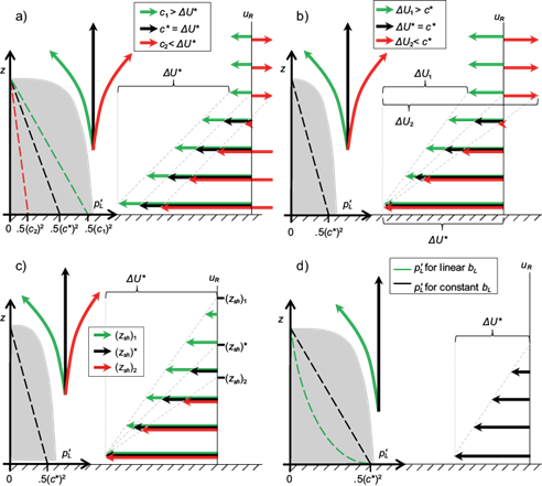
Fig. 2 Schematic illustration of density currents under different environmental conditions and buoyancy profiles: environmental winds are displayed on the right (horizontal arrows), the gray area on the left represents the denser air, on top of which pressure perturbation profiles at L are overlaid (thick dashed lines), and next to which the updrafts diagnosed by MB are displayed (arrows pointing upwards). Each figure represents specific variations of the airflow at L or R around an “optimal” baseline case with c* = ΔU* and MB = 1 (the asterisk indicates baseline parameter values). Baseline profiles are shown in black, while profiles corresponding to LFM > MF (LFM < MF) are in green (red). The effects of performing “classic” c and ΔU variations are displayed in a) and b), respectively, c) shows the impacts of modifying z sh while holding ΔU fixed, and d) depicts a case with a linear buoyancy profile which gives c*.
An important difference between MB and c/∆U is that the former depends on the specific distributions of hydrostatic pressure perturbations at L and environmental winds, while the latter is completely specified by the limit values determining environmental winds aloft: u R,0 , u R,zsh , p' L,0 and p' L (z dc ), although the latter is zero in all cases considered herein. Consequently, MB can differ significantly from c/∆U.
For instance, consider an environment with constant shear below z sh , that is, u R = u R,0 (1 - z/z sh ) for 0 < z < z sh , constant wind velocity aloft, u L = 0, and c/∆U = 1. In this case, solving the integrals in (16) gives LFM = (∆U2/3) z sh , i.e. LFM is directly proportional to the shear-layer depth. Given that greater LFM is associated with downwind updraft tilting, as illustrated in Figure 2c, it is possible that MB can account for BR14’s results revealing the updraft’s sensitivity to the environmental shear-layer depth for cases with c/∆U = 1. Similarly, for given c and z dc , it can be shown that the MF corresponding to a linear b distribution below z dc is lower than the MF for constant b, implying that the former case is more favorable for the development of downwind tilted updrafts (Fig. 2d). This suggests that momentum-balance might also explain updraft sensitivities to the buoyancy distribution within denser air, as documented for density currents (Droegemeier and Wilhelmson, 1987) and MCSs (Alfaro and Khairoutdinov, 2015).
3. Methodology
3.1 Numerical framework
The 2D density current simulations closely follow BR14’s approach to enable us to compare our results to theirs. Numerical experiments are performed with the non-hydrostatic cloud model CM1 version 18 (code and documentation available at http://www2.mmm.ucar.edu/people/bryan/cm1/). The dynamical core is based on the viscous compressible Boussinesq equations. The model is run as a direct numerical simulation (DNS), with Prandtl and Reynolds numbers set to 1 and 104, respectively. The viscous stress and conductivity terms are calculated as in BR14. Upper and lower boundaries are flat, rigid and free-slip, while lateral boundaries are open. The domain is 100 km wide and 20 km deep, with ∆x = ∆z = 50 m grid spacing.
The initial conditions are not entirely consistent with a steady flow in equilibrium. It takes some time for the dense fluid to accelerate and reach a quasi-steady state. Consequently, the simulations are run for 3 h to allow the updrafts to reach quasi-steadiness. This strategy, whereby the dense fluid is initially static, is common practice in time-evolving simulations of density currents (e.g. RKW88, WR04 and BR14).
Initial conditions are prescribed through the buoyancy and vorticity profiles at L and R, respectively, which are extended to the interior of the domain as follows:
where η = ∂u / ∂z - ∂w / ∂x is the horizontal vorticity and x* is the center of the domain. Equations (17) and (18) were chosen based on results by BR14 showing that they produce initial conditions lacking a well-defined updraft and with nearly static denser air (Fig. 3a). The second equality in (18) is determined by the theoretical speed of parcels that follow the density current’s interface under the assumption of strictly vertical pressure gradients therein and Bernoulli energy conservation (the layer of baroclinically generated shear extends 6 grid points, roughly corresponding to the minimum resolvable scale). The third equality in (18), which was not considered in BR14, is included to guarantee that (6) is satisfied at initiation, helping maintain z dc nearly constant throughout the simulation. BR14’s Figures 15-16 show that density currents eventually develop thin layers with vorticity of the same sign as ∆U - c immediately above the denser air. This vorticity is mainly produced baroclinically as z dc changes near the density current’s edge, and it manifests as the flow seeks to satisfy (6) with u L = u R above z max .
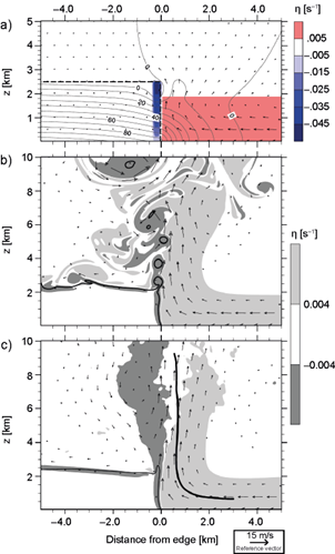
Fig. 3 Fields produced by the baseline simulation. Initial conditions are shown in a), where the vorticity field is indicated by colored contours, thin gray lines contour the pressure perturbation field (every 10 Pa), the thick dashed line outlines the denser fluid, and arrows represent velocity vectors (compare to Fig. 3 in BR14). Instantaneous fields at t = 60 min are displayed in b), with filled contours contrasting regions of positive and negative vorticity, solid contours indicating the -0.015 m s-2 buoyancy level, and wind velocities with magnitude greater than 1 m s-1 depicted by arrows (compare to Fig. 5a in BR14). c) is as b), but with fields corresponding to time-averages of snapshots taken every 2.5 min between 60 min and 180 min, with the mean parcel trajectory indicated by the thick solid line.
The initial wind field is obtained from (18) by solving
where  2 = ∂2/∂x
2
+ ∂2/∂z
2
and ψ is the stream-function of the flow, through which the velocity field is determined by u = ∂ψ / ∂z and w = -∂ψ /∂x. Boundary conditions for (19) are ψ = 0 at the upper and lower boundaries, and ∂ψ / ∂x = 0 at lateral boundaries, the latter implying that w
L
= w
R
= 0. After the wind field is retrieved via (18) and (19), the initial pressure perturbation field is found by solving the diagnostic pressure perturbation equation for inviscid and incompressible 2D fluids (Markowski and Richardson, 2010):
2 = ∂2/∂x
2
+ ∂2/∂z
2
and ψ is the stream-function of the flow, through which the velocity field is determined by u = ∂ψ / ∂z and w = -∂ψ /∂x. Boundary conditions for (19) are ψ = 0 at the upper and lower boundaries, and ∂ψ / ∂x = 0 at lateral boundaries, the latter implying that w
L
= w
R
= 0. After the wind field is retrieved via (18) and (19), the initial pressure perturbation field is found by solving the diagnostic pressure perturbation equation for inviscid and incompressible 2D fluids (Markowski and Richardson, 2010):
where v = (u, w). Boundary conditions for (20) are ∂p' / ∂z = -b at the lower boundary, which guarantees zero vertical acceleration per (2); p' = 0 at the upper boundary, and ∂p' / ∂x = 0 at lateral boundaries. Equation (20) is satisfied by inviscid flows governed by (1)-(4), so it provides reasonable guidance for specifying initial conditions in the present context. Figure 3a shows the initial wind, vorticity and pressure perturbation fields of a density current simulation which develops a vertical updraft by 60 min, as revealed by Figures 3b and 3c.
3.2 Experimental design and the baseline simulation
The experimental design consists of modifications to initial b L and η R profiles (Eqs. 12-13) around a baseline case studied in detail by BR14. The baseline simulation is specified by z sh = 1900 m and ∆U = 15 m s-1, such that η R = ∆U/z sh below z sh , while η R = 0 aloft; also, b L = -0.045 m s-2 below z dc = 2533 m, giving c = 15 m s-1. The resulting initial conditions and simulated fields at 60 min are displayed in Figures 3a-3b. Figure 3b shows that the baseline density current develops a vertical updraft, which is consistent with it having MB = 1 and c /∆U = 1. Given that our simulations are not strictly steady, subsequent analyses focus on time averaged wind fields, as those presented in Figure 3c (the horizontal frame of reference has the origin anchored at the density current’s edge).
To further characterize updrafts, we consider the mean Lagrangian trajectories traced by parcels originating near the surface, as depicted by the solid line in Figure 3c. The mean trajectory is defined as in Alfaro (2017):
where [x(s), z(s)]i is the i-th trajectory parameterized by s, the trajectory length, and N is the number of different parcels used for averaging. Parcels are initialized ahead of the density current edge 60 min into the simulation, when the updraft appears to be well developed (Fig. 3b), being uniformly distributed in space every 2500 m in the horizontal, with heights at 425 m, 625 m, and 825 m. Each trajectory in (21) is initialized by the condition s = 0 when the parcel first arrives at 3 km ahead of the density current edge. Only trajectories that reach s > 10 km at the end of the simulation are used for averaging; however, to evaluate MB we focus on the layer between 1.5 km and 5.5 km height, the lower limit being near the level where the trajectory in Figure 3c first appears vertical, while the upper limit is slightly above the deepest shear-layer considered herein. We consider this layer to be appropriate for characterizing how updrafts are affected by interactions between the negatively buoyant air and the surface-based shear.
4. Results
We analyze the updrafts developed by several simulated density currents, considering the impact of systematically changing one specific characteristic of the flow, everything else being equal. Several parameters describing the simulations are presented in Table I in dimensional form to facilitate comparisons with SLs and their environments. The parameters α and β determine the shear and buoyancy profiles, respectively (subsection 4.2, Eqs. 22-23), with baseline values of α = 1 (constant η R below z sh ) and β = 0 (constant b L below z dc ). As in BR14, values reported in Table I were computed from initial b L and η R profiles, where it is assumed that (6) holds and that u R = u L above z max . We held z dc constant among all experiments, guaranteeing that our simulations are dynamically distinct from each other.
Table I Relevant parameters, determined by initial conditions, of simulated density currents.
| Fig. | 3 | 4a | 4b | 4c | 4d | 4e | 4f | 6a | 6b | 6c | 6d |
| c/∆U | 1.00 | 1.50 | 1.30 | 1.20 | 0.60 | 0.70 | 0.80 | 1.00 | 1.00 | 1.00 | 1.00 |
| MB | 1.00 | 1.56 | 1.33 | 1.22 | 0.60 | 0.70 | 0.80 | 2.60 | 2.00 | 0.66 | 0.83 |
| z sh | 1900 | 1900 | 1900 | 1900 | 1900 | 1900 | 1900 | 5050 | 3800 | 1250 | 1580 |
| α | 1 | 1 | 1 | 1 | 1 | 1 | 1 | 1 | 1 | 1 | 1 |
| β | 0.0 | 0.0 | 0.0 | 0.0 | 0.0 | 0.0 | 0.0 | 0.0 | 0.0 | 0.0 | 0.0 |
| Fig. | 7a | 7b | 7c | 7d | 9a | 9b | 9c | 10a | 10b | 10c | 11a |
| c/∆U | 1.00 | 1.00 | 1.00 | 1.00 | 1.00 | 1.00 | 1.00 | 1.00 | 1.00 | 1.00 | 1.00 |
| MB | 1.50 | 1.20 | 0.60 | 0.75 | 2.00 | 1.50 | 1.25 | 1.00 | 0.75 | 0.63 | 3.60 |
| z sh | 1900 | 1900 | 1900 | 1900 | 1900 | 1900 | 1900 | 950 | 950 | 950 | 3800 |
| α | 0.5 | 0.75 | 2 | 1.5 | 1 | 1 | 1 | 1 | 1 | 1 | 0.75 |
| β | 0.0 | 0.0 | 0.0 | 0.0 | 2.0 | 1.0 | 0.5 | 2.0 | 1.0 | 0.5 | 1.0 |
| Fig. | 11b | 12a | 12b | 12c | 12d | 12e | 12f | 13a | 13b | 13c | 13d |
| c/∆U | 1.00 | 0.70 | 1.33 | 0.80 | 1.35 | 0.67 | 1.20 | 0.60 | 1.50 | 0.75 | 1.20 |
| MB | 0.50 | 1.00 | 1.00 | 1.00 | 1.00 | 1.00 | 1.00 | 1.00 | 1.00 | 2.40 | 0.70 |
| z sh | 1250 | 5050 | 1250 | 1900 | 1900 | 1900 | 950 | 3800 | 1250 | 3800 | 1250 |
| α | 1.5 | 1 | 1 | 0.75 | 2 | 1 | 1 | 0.75 | 1.5 | 0.75 | 1.5 |
| β | 0.0 | 0.0 | 0.0 | 0.0 | 0.0 | 1.0 | 1.0 | 1.0 | 0.0 | 1.0 | 0.0 |
4.1 “Classic” ∆ U variations
This subsection considers the effect of varying the constant determining η R below z sh , everything else being equal (Fig. 2b). These classic inter-case variations are analogous to those contemplated by RKW88, WR04, and BR14. We do not show cases where c is varied, as we find that updrafts respond in analogy to ∆U variations as a function of c/∆U, in agreement with BR14.
Figure 4 shows results corresponding to six simulations, three with 1 < c/∆U ≤ 1.5 (Figs. 4a-4c) and three having 0.6 ≤ c/∆U < 1 (Figs. 4d-4f). As in previous investigations, flows with 1< (>) c/∆U develop downwind (upwind) slanted updrafts, following the direction of environmental winds aloft. That c/∆U ≈ MB in each simulation implies that both metrics vary in concert under classic ∆U variations, which explains the large sensitivity of the updraft slope to changes in the shear’s strength (the same is true for c variations; not shown). Also note that simulations with downwind (upwind) tilted updrafts develop vortices on the downwind (upwind) side of the density current’s edge, a feature that is common to many simulations considered in latter subsections. These circulations complicate the interpretation of the rhs of (13) as a measure of the updraft’s orientation, while the fact that they induce non-hydrostatic pressure perturbations and alter wind velocities suggests that caution must be exercised when defining the control volume to compute MB.
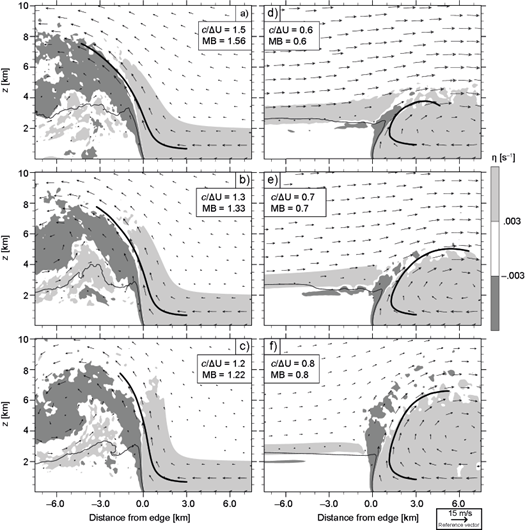
Fig. 4 As Figure 3c, depicting cases with varying ΔU (subsection 4.1). For reference, each figure displays the corresponding c/ΔU and MB (see Table I).
Instantaneous fields at 30 min are shown in Figure 5, revealing the association between the aforementioned circulations and non-hydrostatic pressure perturbations. As expected from (20), vortices are centered on p' < 0, while flow deformations occur within p' > 0 (Markowski and Richardson, 2010, pp. 27-28), e.g. at the rightmost edge of Figs. 5e, where air that previously exited the updraft encounters inflowing environmental air. It is worth noting that these features reach lateral boundaries late in the simulations, affecting the instantaneous computation of MB. This, however, does not undermine our results, as we found little sensitivity in time averaged fields and mean trajectories when the simulations with c/∆U = 1.5 (Fig. 4a) and c/∆U = 0.6 (Fig. 4f) were performed in a domain twice as large (not shown). In fact, the case-by-case similarity between updrafts at 30 min (Fig. 5) and the time averaged updrafts (Fig. 4) suggests that the flow’s structure near the density current’s edge is established early in the simulation, remaining quasi-steady thereafter. These considerations, which apply to all simulations considered herein, justify our interpretation of time averaged fields and mean trajectories through the MB computed from initial conditions.
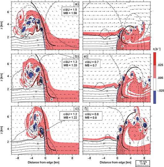
Fig. 5 Instantaneous pressure perturbations (contour lines; dashed for negative values), wind velocities (arrows), and vorticity field (colors) at 30 min corresponding to the simulations in Figure 4. Mean trajectories are included for reference.
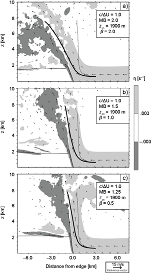
4.2 Simulations with c/∆ U=1
First, we consider the effects of varying z sh in cases with baseline’s ∆U satisfying c/∆U = 1. Simulations in Figure 6 have z sh varying between 2(z dc )=5050 m (Fig. 6a) and 0.5(z dc ) = 1,250 m (Fig. 6c), showing that shallow (deep) shear layers favor upwind (downwind) updraft tilting. The variety of updraft structures in Figure 6 demonstrate that c/∆U does not provide accurate guidance on the density-current-shear interactions that modulate the ascent of near-surface air. On the other hand, updraft slopes vary systematically as a function of MB, in agreement with Figure 2c, suggesting that momentum-balance captures relevant features to which c/∆U is insensitive. Also note that vortices resembling those in Figure 4 appear on the updraft’s flank determined by its slope, showing that these circulations arise independently of the value of c/∆U.
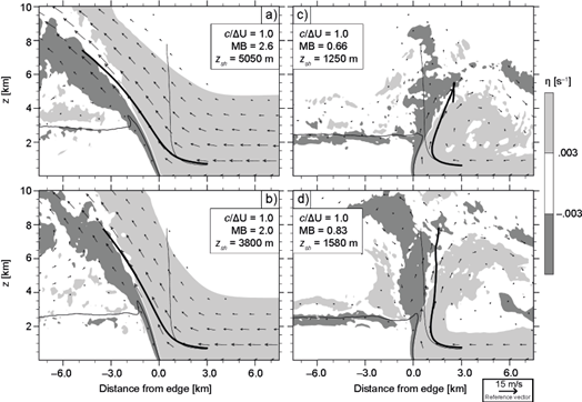
Fig. 6 As Figure 4, depicting cases with varying z sh (subsection 4.2). The thin line indicates baseline’s mean trajectory.
Figure 7 shows results from density currents in environments with non-constant shear below a fixed baseline’s z sh . The u R profiles used for these simulations are displayed in Figure 8a, which were determined by
where α = 0.5 (Fig. 7a), 0.75 (Fig. 7b), 2 (Fig. 7c), and 1.5 (Fig. 7d). Note that (22) can produce different LFM for given ∆U and z sh (Eq. 16). It is readily seen in Figure 8a that environmental wind speeds within the shear-layer are a decreasing function of α, such that greater α is associated with lower LFM and MB. Consistent with the value of MB, and notwithstanding c/∆U = 1, greater momentum inflow at R favors downwind updraft tilting (Figs. 7a-7b), while weak inflow leads to upwind sloping updrafts (Figs. 7c-7d).
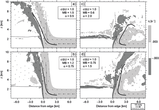
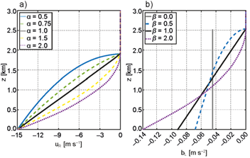
Fig. 8 In a) environmental wind profiles with baseline’s z sh and ΔU derived from (22). In b) varying buoyancy profiles as determined by (23). The gray line denotes the constant b 0 corresponding to the baseline case.
Simulations depicted in Figure 9 have varying b L profiles with baseline’s c and u R . From hydrostaticity at L, buoyancies are expected to affect MB via the MF (rhs of Eq. 14). The buoyancy profiles considered herein, shown in Figure 8b, were specified as follows:
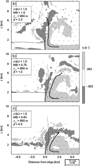
where β = 2 (Fig. 9a), 1 (Fig. 9b), and 0.5 (Fig. 9c); and b 0 is the surface buoyancy required for baseline’s c. It is easy to show that MF (MB) is a decreasing (increasing) function of β, in agreement with the downwind tilted updrafts in Figure 9 (β = 0 in baseline), with greater slopes corresponding to larger β. Analogously, fields in Figure 10 demonstrate that, for given c and u R , updrafts can tilt upwind in response to changes in b L . Simulations in Figure 10 have z sh = 950 m, which gives MB = 1 in the case where β = 2. Thus, the density current in Figure 10a is momentum-balanced, consistent with its vertical updraft, while cases in Figures 10b-10c have lower MB (higher MF), in agreement with their upwind tilted updrafts.
Finally, we consider the combined effects of varying u R and b L to produce MB that differs significantly from 1 for c/∆U = 1. Results in Figure 11a correspond to a case with baseline’s c and ∆U, but with z sh = 3800 m, α = 0.75, and β = 0.75, giving MB = 3.6. Fields in Figure 11b were produced by a simulation with z sh =1266 m, α = 1.5, and β = 0, giving MB = 0.5. These two density currents have the most pronounced updraft slopes among all cases considered, consistent with their contrasting MB, and notwithstanding both having c /∆U = 1. This result highlights the importance of processes ignored by c/∆U but measured by MB. This, and the fact that vertical updrafts arise when z sh is adjusted to satisfy MB = 1, as revealed by Figure 10a and shown by BR14 for varying shear profiles (see their Fig. 19), supports the momentum-balance concepts discussed in subsection 2.3 and illustrated in Figure 2.
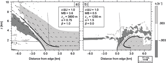
Fig. 11 As Figure 6, depicting cases with combined z sh , u R (z) and b L (z) profile variations (subsection 4.2).
4.3 Simulations with MB=1 and c/∆U≠1
This subsection analyzes momentum-balanced density currents based on cases analyzed in the previous subsection. Specifically, ∆U is varied to satisfy MB = 1, while holding c, z sh , α, and β fixed. We consider the following simulations: cases with z sh values of 5050 m (Fig. 12a; compare to Fig. 6a) and 1250 m (Fig. 12b; compare to Fig. 6b); with α equal to 0.75 (Fig. 12c; compare to Fig. 7b) and 2 (Fig. 12d; compare to Fig. 7c; α = 0.5 is not shown because it developed vortices due to Kelvin-Helmholtz instability); the two cases with β = 1 (Figs. 12e-12f; compare to Figs. 9b and 10b), as linear b profiles are relevant to SLs (RKW88; WR04); and the two cases with combined effects (Figs. 13a and 13b, compare to Figs. 11a and 11b, respectively).
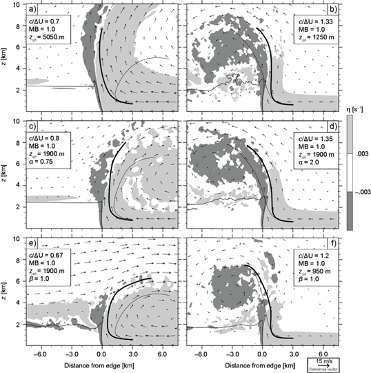
Fig. 12 As Figure 4, depicting cases with MB = 1 and varying c/∆U (subsection 4.3). The thin line indicates the mean trajectory produced by the case in Figure 4 with the closest corresponding value of c/∆U.
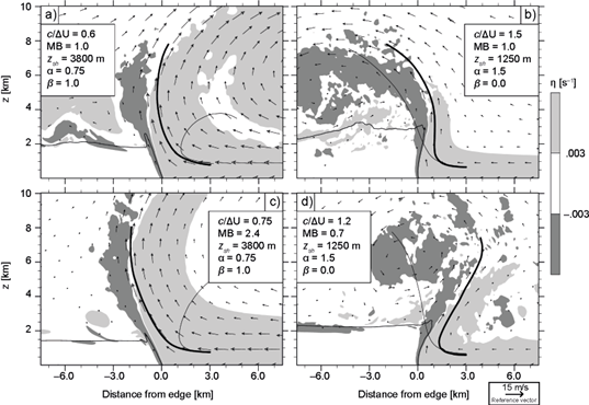
Fig. 13 As Figure 12, depicting cases with combined z sh , u R (z) and b L (z) profile variations (subsection 4.3).
Figure 12 shows that most updrafts are nearly vertical throughout low and mid-levels, especially if a case-by-case comparison is made with the mean trajectory of the simulation having the most similar c/∆U among the density currents described in subsection 4.1 and illustrated in Figure 4 (e.g. Fig. 4e and Fig. 12a both have c/∆U = 0.7). In other words, at low levels, updrafts tend to become vertical for MB ≈ 1, despite c/∆U ≠ 1; at upper-levels, updrafts tilt in the direction of environmental winds aloft, as diagnosed by c/∆U. Note that the tilt at upper levels determines the updraft’s flank where noticeable vortices develop, which in turn could have minor effects on the updraft’s slope at low and mid-levels, e.g. the modest upwind slopes at low levels in Figures 12d-12e.
Figure 13 further exemplifies the behavior described above, wherein the case with MB = 1 in Figure 13a (13b) should be contrasted with its counterpart in Figure 13c (13d), the latter having MB > (<) 1 and c/∆U < (>) 1, i.e. opposing MB and c/∆U: the updraft of the former is nearly vertical at low levels, tilting aloft in the direction determined by c/∆U; in the latter, the updraft tilts downwind (upwind) at low levels, as determined by MB, changing its direction aloft in accordance with c/∆U. We consider these results and those presented in the previous subsection to be strongly indicative of the fact that c/∆U is more appropriate as a measure of the tendency of the updraft to tilt in the direction of environmental winds aloft, rather than near-surface density-current-shear interactions, for which MB seems to be better suited.
4.4 Updraft orientation and lifting of environmental air for all simulated density currents
Results presented above consistently indicate that MB can account for the impacts of the shear and buoyancy profiles on the updraft’s orientation throughout low and mid-levels. To get a broader perspective of this result, the mean trajectories of all previously described simulations are shown in Figures 14a-14b. Each trajectory is translated horizontally such that x(s) = 0 for s satisfying z(s) = 1.5 km (Eq. 16), which facilitates comparing among different updraft slopes between 1.5 km and 5.5 km height. Curves are colored per MB-1 in Figure 14a, and per ΔU/c in Figure 14b, where the reciprocal is used because it provides greater symmetry of index values around 1. Updraft slopes appear to be in close correspondence with MB, but there is no indication of such a relation with c/ΔU. Another way to visualize this result is by looking at scatterplots where the ordinate axis indicates the horizontal position of the trajectory at 5.5 km height, denoted by x 5.5 , and either MB-1 or ΔU/c in the abscissa axis (Figs. 14c-14d). An extrapolation is made to compute x 5.5 in cases where the updraft does not reach 5.5 km height, assuming the slope between 1.5 km and the trajectory’s maximum height is constant up to 5.5 km.
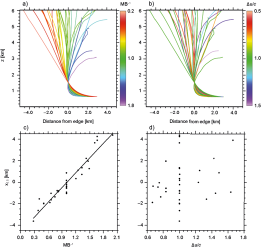
Fig. 14 In a) and b) the mean trajectories of all simulations are displayed up to their maximum height. Trajectories are colored by the simulation’s MB-1 in a) and ΔU/c in b). The scatter plots in c) and d) show all simulations per their MB-1 and ΔU/c in the abscissa axis, and x 5.5 in the ordinate axis. The line in c) corresponds to the best linear fit to the data.
In Figure 14c there appears to be a linear correspondence between MB-1 and x 5.5 , with momentum- balanced simulations (MB-1 = 1) spanning a relatively narrow range of slopes around x 5.5 = 0. On the other hand, Figure 14d does not reveal any obvious functional relation between ΔU/c and the updraft slope, with simulations having static environmental winds aloft spanning the entire range of simulated x 5.5 .
In addition to the updraft slope, we are interested in analyzing the depth reached by near-surface environmental air, a matter that is central to RKW theory (Bryan et al., 2012), for which WR04 and BR14 found ΔU/c to be an effective diagnostic. We follow WR04 and BR14 by specifying a passive tracer, tr, initialized as tr(x, z, t0) = z at t 0 = 60 min; its maximum displacement at t 1 = 90 min being defined as δ max = max{z - tr(x, z, t1)│tr < 1 km}. Results are presented in Figure 15, wherein the ordinate axis specifies δ max , while the abscissa corresponds to either MB-1 or ΔU/c (Figs. 15a-15b).
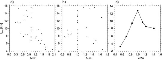
Fig. 15 Scatter plots showing δ max (ordinate). All simulations are displayed in a) and b), where the abscissa indicates MB-1 and ΔU/c, respectively. The scatter plot in c) displays c/ΔU- δ max for “classic” variations (compare to BR14’s Fig. 17).
Figure 15a shows that cases with MB = 1, which have the most vertical updrafts (Figs. 14a and 14c), do not necessarily produce the deepest lifting of environmental air. Yet, near-surface air tends to reach deeper in cases with large MB, implying that systems with downwind tilted updrafts are the most effective at lifting environmental air. It appears that greater momentum inflow at R is associated with deeper updrafts (e.g. Figs. 6a, 6b, 7a, 7b, 11a, which have large z sh or α < 1, or both), perhaps because greater system-relative mass inflow enables broader circulations near the density current’s edge than when the inflow is weak. This behavior is consistent with the notion that deep shear-layers favor the lifting of near-surface environmental air high into the upper-troposphere, as suggested by Coniglio et al. (2006). However, a more detailed analysis of the relationship between inflowing air and of the depth of the updraft is beyond the scope of this work.
Figure 15b does not reveal a close relation between the depth reached by near-surface environmental air and ΔU/c. In order to validate this finding, we performed additional simulations with varying c to create Figure 15c, which shows results consistent with those in BR14’s Figure 17, wherein near-surface parcels reach deeper in cases with c/ΔU closer to 1. Therefore, while c/ΔU seems to be an effective diagnostic under classic c variations, under more general conditions the environmental wind speed aloft is not an effective diagnostic of a density current’s ability to lift near-surface air.
5. Discussion
5.1 Merits and limitations of momentum-balance in density currents
Our results show that momentum-balance can be effective for diagnosing the orientation of updrafts in density currents, accounting for “classic” c-∆U variations, the shear-layer depth, the shear profile, and buoyancies within the denser air. It is true that the experiments considered herein include a limited set of initial conditions, so generalizations could warrant caution, especially in no-shear environments, which were not contemplated since they are not very relevant to SLs’ organization. Yet, the robustness of our results is substantiated by the fact that the numerical experiments considered herein mirror those contemplated by BR14 (except for buoyancy profile variations, which were not included in that study), guaranteeing that our methodology was not designed to favor MB over c/ΔU. Furthermore, this study considers more diverse variations to environmental winds and buoyancy profiles than previous analyses of density currents aimed at understanding SL-shear interactions (RKW88; WR04; BR14). We are thus led to the conclusion that momentum-balance represents an effective conceptual framework for characterizing the slope of a density current’s updraft throughout low and mid-levels, which is advantageous over RKW’s quantitative criterion for its greater ability to account for varying shear and buoyancy profiles.
It is important to mention that only modest changes around c/∆U = 1 were contemplated in this study. This is so because cases of relevance to SL environments where c/∆U differs significantly from 1 produce updrafts with pronounced slopes in the direction of winds aloft. This is due to the underlying relationship between MB and c/∆U, as exemplified by considering classic ∆U variations: both MB and c/∆U vary in concert in response to changes in ∆U (Fig. 2b; subsection 4.1), implying that the airflow aloft and momentum-balance interactions between the denser air and inflowing winds tend to tilt the updraft in the same direction. However, it does not follow that MB only provides relevant information in cases with c/∆U ≈ 1, especially in SLs, which develop significant within-storm pressure perturbations above the cold pool (Fovell and Ogura, 1988; Lafore and Moncrieff, 1989), directly affecting the MF. Such features, together with non-stagnant air within the cold pool, can strongly affect the system-relative inflow through the propagation speed (Trier et al., 2006; Mahoney et al., 2009), suggesting that c/∆U might not provide reasonable guidance for system-relative winds aloft.
There are two issues that deserve further note: circulations affecting the momentum structure near the updraft and the neglect of outflowing momentum at lateral boundaries of the control volume. Regarding the former, vortices flanking the updraft are likely to have an impact on ascending motions, even though in cases considered herein they do not significantly affect the diagnostic skill of MB. Perhaps more relevant are the circulations associated with non-hydrostatic pressure perturbations that reach lateral boundaries, complicating the definition of L and R. However, as mentioned in subsection 4.1, relevant characteristics of the updrafts seem to be established early in the simulations, justifying the use of initial conditions to compute MB. On the other hand, such features are not likely to be relevant to SLs, the phenomenon motivating this study, wherein stably stratified environmental and within-storm conditions should damp those circulations, guaranteeing nearly hydrostatically balanced flow at lateral boundaries.
The neglect of outflowing momentum at lateral boundaries might seem ad-hoc for the density currents considered herein, as there is no formal argument based on the momentum theorem (Batchelor, 2000) for defining LFM as in (16). The problem arises because the momentum theorem does not represent an equation for the updraft’s slope, although there clearly exists a close relationship between the momentum structure at lateral boundaries and updraft characteristics. We believe that the physical plausibility of our arguments, wherein inconsistencies arise between the foreseen effects of outflowing air and the mathematical expressions derived from the momentum theorem (subsection 2.3), substantiate our definition of the LFM, while results presented throughout section 4 provide strong support for this choice. It is worth noting that WR04 and BR14 proceeded in this way (see Bryan et al., 2012), i.e. first providing plausible qualitative arguments relating the updraft’s structure to the quantitative criterion derived from a single “optimal” density current, and then validating numerically the applicability of c/∆U to non-optimal cases. Therefore, considering that this is not a study about the momentum theorem in diverse density currents, we think that the momentum-balance concepts discussed are appropriate means for diagnosing the updraft’s orientation throughout low and mid-levels, as long as physical arguments and numerical evidence support this interpretation.
5.2 RKW theory and the reinterpretation of the quantitative criterion
One of the most surprising findings of this investigation is the lack of correspondence between the quantitative criterion of RKW theory and both the updraft’s slope and the depth reached by near-surface environmental air. We believe that the close correspondence between MB and c/∆U under classic c-∆U variations led previous studies to misidentify c/∆U as an accurate measure of near-surface density-current-shear interactions. This is further substantiated by the fact that the vorticity-balance relation in (11) does not show a clear relationship with c/∆U for non-optimal configurations.
In addition, results presented in section 4 lend weight to our reinterpretation of c/∆U as a measure of the impacts of winds aloft on the updraft’s structure. Such effects are akin to those contemplated by Thorpe et al. (1982) in the context of SLs, wherein the movement of the cold pool edge relative to previously triggered deep convective cells is of primary importance to the organization and maintenance of storms. The importance of system-relative winds aloft lies in their ability to tilt the top of the updraft, which may be the result of the airflow impinging on ascending parcels with near-surface origins. This effect was recognized by Shapiro (1992) and Coniglio et al. (2006) in flows with deep shear-layers. Thus, we are inclined to interpret c/∆U as a measure of an updraft’s tendency to slope in the direction of the wind velocity aloft, instead of the near-surface interactions between the density current and inflowing winds, as originally intended by RKW88. For clarity, we do not deny that c/∆U is related to the near-surface vorticity field in the updraft’s vicinity, but these theoretical considerations and results presented lead us to conclude that c/∆U does not provide an accurate measure of the near-surface density-current-shear interactions considered by Rotunno et al. (1988), Weisman and Rotunno (2004), and Bryan and Rotunno (2014).
It is worth mentioning that this interpretation of c/∆U fits within the momentum framework, with winds aloft “pushing” the updraft in the direction determined by c/∆U. Therefore, we interpret MB as a momentum-balance metric for near-surface interactions between the density current and inflowing air, while c/∆U provides information on the impact of wind velocity alofton the updraft.
6. Summary and future work
This study presents a momentum-balance framework for diagnosing the slope of a density current’s updraft in sheared environments, pursuing a theory of storm-shear interactions that can bridge gaps in the RKW theory of vorticity-balance. The motivation arose from results by BR14 showing that the quantitative criterion of RKW theory, c/ΔU, cannot account for the impacts of shear-layer depth variations on a density current’s updraft, while also demonstrating the importance of the flow-force balance constraint (Benjamin, 1968) for the development of the optimal state. Given that the flow-force balance represents a condition on the horizontal momentum equation determining the shear-layer depth for the optimal state, momentum-balance concepts are explored as an alternative to RKW theory.
We derived a non-dimensional quantitative diagnostic concerning the degree of momentum-balance (MB) for density currents, which depends on both the shear and buoyancy profiles. MB measures the extent to which hydrostatic pressure perturbations within the denser air-which favor upwind tilted updrafts-can counter advective tendencies due to inflowing environmental air-which favor downwind tilted updrafts. We evaluate the diagnostic skill of MB by comparing the updrafts produced by several numerically simulated density currents, wherein profiles of environmental winds and buoyancies within the denser fluid were varied systematically from case to case. Results show that MB can effectively diagnose the updraft’s slope throughout low and mid-levels, accounting for classic c-ΔU variations, changes to the shear-layer depth, and varying buoyancy and shear profiles.
Regarding RKW theory, our results show that c/ΔU is not as restrictive on a density current’s updraft as suggested by previous investigations (RKW88; WR04). In particular, we do not find a clear relationship between c/ΔU and either the low-to-mid level updraft slope or the lifting of near-surface air. This could be due to c/ΔU not being an accurate measure of vorticity-balance in non-optimal density currents. On the other hand, the close correspondence between c/ΔU and environmental wind velocities at upper levels lead us to reinterpret c/ΔU as a measure of the impacts of the airflow aloft on the updraft. Consistent with this interpretation, updraft slopes at upper levels follow the direction of the environmental winds aloft, as determined by c/ΔU.
It is early to guarantee the application of MB concepts to observed SLs, but lateral flux of momentum (LFM) can be computed from data analysis by estimating the system’s propagation velocity, e.g. by using Corfidi vectors (Corfidi, 2003) to provide additional information in understanding SLs organization. The motive force (MF) term is more difficult to estimate because it requires knowledge about characteristics within the storm, which are hard to measure. However, the layer lifting model of convection by Alfaro (2017) produces indices, that could be used to approximate within-storm characteristics.
Future research will focus on the validation of momentum-balance concepts in numerically simulated SLs. First, by diagnosing a SL’s evolution throughout early stages, and second, by comparing the updraft structures developed by mature storms in diverse environmental conditions. It is expected that momentum-balance will provide a useful framework for incorporating the circulations within the cold pool in SLs with trailing-stratiform precipitation.

