


Servicios Personalizados
Revista
Articulo
 Inglés (pdf)
 Artículo en XML
 Referencias del artículo
 Enviar artículo por email
Indicadores
-
 Citado por SciELO
 -
 Accesos
Links relacionados
-
 Similares en
SciELO
Similares en
SciELO
Compartir

 Permalink
Atmósfera
versión impresa ISSN 0187-6236
Atmósfera vol.20 no.2 Ciudad de México abr. 2007
Interannual and interdecadal variability in the predominant Pacific
region SST anomaly patterns and their impact on climate in the
mid–Mississippi valley region
A. R. LUPO, E. P. KELSEY, D. K. WEITLICH, J. E. WOOLARD
Department of Soil, Environmental, and Atmospheric Science
302 E Anheuser Busch Natural Resources Building
University of Missouri – Columbia
Columbia, MO, USA 65211
Corresponding author: A. R. LUPO; e–mail: LupoA@missouri.edu
I. I. MOKHOV
Laboratory of Climate Theory, A. M. Obukhov Institute of Atmospheric Physics
Russian Academy of Sciences Pyzhevsky, 119017, Moscow, Russia
P. E. GUINAN
Missouri Climate Center, 1–74 Agriculture Building
University of Missouri – Columbia, Columbia, MO, USA 65211
F. A. AKYÜZ
North Dakota State Climatologist
209 Walster Hall, North Dakota State University,
Fargo, ND, USA 58105
Received January 25, 2006; accepted August 28, 2006
RESUMEN
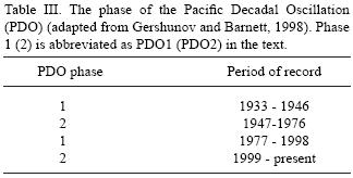
Estudios previos han demostrado que las temperaturas en la superficie del mar (SSTs) y las anomalías de temperatura de la superficie del mar (SST) en la región del Pacífico pueden clasificarse en siete patrones o conglomerados (A–G). Los conglomerados B y G (C, D y F) [A y E] son representativos de distribuciones SST en periodos de La Niña (El Niño) [neutral]. El análisis de patrones SST para el periodo 1955–1993 ha demostrado que los conglomerados A–D fueron predominantes en el primer periodo 1955–1977, mientras que los tipos E y F dominaron en el último periodo de estudio. Los conglomerados tipo G fueron poco frecuentes pero ocurrieron durante ambos periodos. Este cambio en la frecuencia de patrones durante 1977 corresponde a cambio de fase de la Oscilación Decadal del Pacífico (PDO). En este estudio se lleva a cabo un análisis similar extendido al periodo 1994–2005. Los resultados revelan un cambio en los patrones predominantes de SSTs asociado a un cambio simultáneo en la fase de la PDO durante 1999 y 2000. Los patrones SST evolucionaron desde unas anomalías predominantemente de tipo E y F en 1994 a anomalías de tipo A, B, D y G en 2005. Estos resultados sugieren que los conglomerados A–D (C, D y F) son característicos de fases negativas (positivas) de la PDO. Por otro lado, el empleo de una técnica modificada para generar diagramas de fase muestra la existencia de variaciones interanuales e interdecadales en la temperatura media mensual y en los registros de precipitación de la región central del Mississippi que pueden asociarse con ENSO y la PDO. Además, un análisis de la asociación estadística entre anomalías de temperatura y precipitación en la región central de Mississippi, y regímenes prolongados de SST revela que las anomalías B, D y G se asociaron con condiciones cálidas, mientras que las anomalías de tipo C y E lo hicieron con condiciones frías. Las anomalías C, D, F y G se asociaron con condiciones más secas de lo normal.
ABSTRACT
Previous research has demonstrated that Pacific Region SSTs and SST anomalies can be separated into seven general synoptic classifications (clusters) (A–G). Clusters B and G (C, D, and F) [A and E] were shown to be generally representative of La Niña (El Niño) [neutral] type SST distributions. Further, an analysis of the SST patterns in 1955–1993 demonstrated that clusters A–D were prominent in 1955–1977, while types E and F dominated the later period. Type G clusters were comparatively rare, but occurred during both periods. In retrospect, this shift during 1977 corresponds roughly with a change in phase of the Pacific Decadal Oscillation (PDO). After updating the analysis to include the 1994 to 2005 period, there was a corresponding change in the predominant SSTs associated with a change in phase of the PDO during 1999 and 2000. The results show that SST patterns did evolve from predominantly E and F–type anomalies in 1994 to A, B, D and G–type anomalies through 2005. Thus, these results suggest that A through D–type (C, E, and F–type) SST clusters are characteristic of the negative (positive) phase of the PDO. Also, using a modified technique for generating phase diagrams, it is shown that there are interannual and interdecadal variations in the mid–Mississippi region monthly mean surface temperature and precipitation records that can be associated with the ENSO and PDO. Additionally, an analysis was performed to see if there was any statistical association between temperature and precipitation anomalies in the mid–Mississippi region and prolonged SST regimes. B, D and G anomalies were associated with warmer–than–normal conditions, while C and E type anomalies tended to be associated with cooler–than–normal conditions across the region. C, D, F, and G anomalies were associated with drier than normal conditions.
Keywords: Interannual variations, El Niño, sea surface temperatures, climate, climate variations.
1. Introduction
Many recent studies have attempted to link variations in global circulation changes (Wallace andGutzler, 1981; Hoskins et al., 1983; Gray et al., 1992; Mantua et al., 1997; Mokhov et al., 1997; Gershanov and Barnett, 1998; Enfield and Mestas–Nuñez, 1999; Mestas–Nuñez and Enfield, 1999; 2001; Weidenmann et al., 2002), or local (and regional) climate variations (Keables, 1992; Kung and Chern, 1995 [hereafter KC95]; Kunkel and Angel, 1999; Berger et al., 2003; Fye et al., 2003; Mokhov et al., 2004) with interannual and interdecadal variations in sea surface temperatures (SSTs) and pressures in the Pacific Ocean basin and/or the changes in the character of the atmospheric and oceanic circulations in the Atlantic Ocean basin (Hu et al., 1998; Lupo and Johnston, 2000; Shabbar et al., 2001). The interactions between the atmosphere and oceans are important processes to consider when attempting to either understand the relevant physics of the earth's climate system or make long–range forecasts (Barnston et al., 1994, 1999; Anderson et al., 1999). The atmosphere and oceans are two important components of the climate system that are considered to be thermodynamically open as they exchange both, heat and mass (Piexoto and Oort, 1992).
The strongest interannual variations in global and regional climate characteristics are largely influenced by El Niño and Southern Oscillation (ENSO) modes (Arpe et al., 2000; Houghton et al., 2001; Mokhov et al., 2000, 2004). Diagnosing regional and local climate variability has been a topic of interest lately, since global circulation models are used heavily to study the potential for climate change (Houghton et al., 2001). Thus, it is critically important that these models are capable to demonstrate that they can simulate not only the range of regional and local climates, but the interannual and interdecadal variations as well. It is well known that anomalous tropical SST distributions have a large impact on the weather and climate by changing heat and mass distributions of the troposphere. Through this influence, anomalous tropical SSTs can ultimately alter the prevailing wind patterns over a large portion of the globe (Namias 1982, 1983; Hoskins et al., 1983; Keables et al., 1992; Gray et al., 1992; Vincent, 1994; Nakamura et al., 1997; Enfield and Mestas–Nuñez, 1999; Mestas–Nuñez and Enfield, 1999, 2001; Renwick and Revell 1999; Wiedenmann et al., 2002 ). This in turn can impact on the frequency, occurrence, and intensity of such phenomena as mid–latitude cyclones (Key and Chan, 1999), tropical cyclones (Gray, 1984; Lupo and Johnson, 2000) and blocking anticyclones (Wiedenmann et al., 2002). However, there are studies (Mestas–Nuñez and Enfield, 2001; Kushnir et al., 2002) that point out that mid–latitude SSTs may not be very influential on mid–latitude circulations. It is well known that the atmospheric boundary layer will tend to equilibrate with the underlying SSTs. As Kushnir et al. (2002) showed in their study, however, the synoptic atmospheric variability will dominate in the mid–latitudes.
KC95 used principal component analysis to extract the large–scale modes of monthly mean global SST anomalies and the Northern Hemisphere tropospheric circulation anomalies during the period 1955–1993. A similar analysis was performed by Enfield and Mestas–Nuñez (1999) and Mestas–Nuñez and Enfield (1999, 2001), but using data covering a period from 1870 to 1991. The KC95 study provided an archive which can be used as guidance for long–range forecasting applications (e.g., forecasting by the use of analogs). A by–product of this analysis demonstrated that global SST anomalies could be classified into one of seven distinct pattern types of anomaly distributions (A–G). Each of these was correlated with corresponding Northern Hemisphere tropospheric mass distributions or flow anomalies, and in subsequent work, correlated with regional surface climatic characteristics (Lee and Kung, 2000). It is noted here, however, that the correlation between SSTs and atmospheric flow patterns do not address any cause and effect for these linkages. KC95 also noted that anomaly types (clusters) A, B, E, and G (C, D, and F) are representative of La Niña or neutral (El Niño) type SST distributions within the Pacific Ocean basin. They also demonstrated that clusters A–D dominated the early portion of their study period (1955–1977), while E and F type clusters dominated the latter portion (1977–1993). G–type SST anomalies were comparatively rare in either period in the KC95 study.
Thus, this work has two primary objectives. The first is to demonstrate the application of the methodologies found in Mokhov et al. (2000, 2004) (see also Mokhov,1995; Mokhov and Eliseev, 1998) to a local time series of monthly mean temperature and precipitation records, with a simple but beneficial modification of the technique. These techniques will demonstrate that there is significant ENSO–related interannual and interdecadal variability found in the local time series. The interdecadal variability will be shown to be likely related to the influence of the Pacific Decadal Oscillation (PDO) (Minobe, 1997; Mantua et al., 1997; Gershunov and Barnett, 1998). The second objective is to extend the KC95 classification study from 1993 to 2005, and this work will demonstrate that the interdecadal variability in SST clusters may also be related to the PDO. In meeting the second objective, we hope to provide useful information and guidance for long range forecasting applications in our region and in an operational environment. This work will also demonstrate that there are statistical relationships between individual SST types and local variations in a raw sample station temperature and precipitation records but that the statistical relationships may not be straightforward.
2. Data and methodologies
2.1 Data
The analyses used in this study were the global monthly mean extended and reconstructed SSTs and SST anomalies compiled by the National Centers for Environmental Prediction (NCEP) and available through the National Oceanic and Atmospheric Administration (NOAA) online archive (http://www.cdc.noaa.gov/cdc/data.ncep.oisst.v2.html. Monthly SSTs and anomalies are available and these can also be found in the monthly Climate Diagnostics Bulletin (www.cpc.ncep.noaa. gov), and the mean SST anomalies in the ENSO region are available from 1864 to the present through the Center for Ocean and Atmospheric Prediction Studies (COAPS – www.coaps.fsu. edu). The 500 hPa heights and height anomalies from the NCEP re–analysis project (Kalnay et al., 1996) were also examined and are available via the many of the same sources referenced above. Finally, the mean monthly temperature and precipitation records for the Columbia Regional Airport (1955–2005) were provided through the Missouri Climate Center and the Midwestern Regional Climate Center. This represents a continuous record for each variable; however, the airport did change location around 1970. This station moved approximately 25 km southward, but there are no indications that this move resulted in significant changes in the climatology (see also Fig. 1). Degrees Fahrenheit and inches are used for the analysis of monthly mean surface temperatures and precipitation since these are still the standard units used for archival of these monthly records and are still the standard for US surface observations. Also, the precise units of the data used in this analysis were not germane to the analysis or discussion presented here.
2.2 Analysis of monthly mean temperature and precipitation
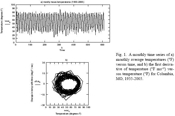
The techniques used here to extract interannual and interdecadal variability from a one–dimensional time series are described by Mokhov et al. (2000, 2004) (and references therein) and will be briefly presented here with modification. The techniques used in these references are based on standard dynamic analysis techniques for physical systems (e.g., Lorenz, 1963). Here we use the time series of temperature and precipitation for Columbia, Missouri, and use this as an example of the analysis technique and the improvement discussed below. The basis for this analysis is derived by constructing simple phase plots of the first derivative of the time series versus the time series itself. If ideally, the function represented by the cyclic time series is sinusoidal (or approximately sinusoidal),
X(t) = A (t) sin [ω(t) + Φ (t0) ] (1)
where X(t) represents a time series of some variable, A (t) the amplitude, and ω(t) the frequency, and Φ(t0) the initial phase, then X(t) from equation (1) represents a general solution to a Sturm–Liouville (oscillator) equation of form,
 + ω2 X = 0 (2)
A simple two–dimensional phase plot of the first derivative versus the time series itself will yield a circular set of trajectories about some mean state (Fig. 1b). In Figure 1, the monthly mean temperatures from 1955–2005 for Columbia, were, as expected, strongly influenced by the annual cycle (Fig. 1a) and represent an approximately harmonic process. The first derivative of monthly mean temperatures (Fig. 1b) was calculated using second order finite differencing, and higher order finite differencing (e.g., 4th order, not shown here) yielded similar, but not necessarily more robust results.
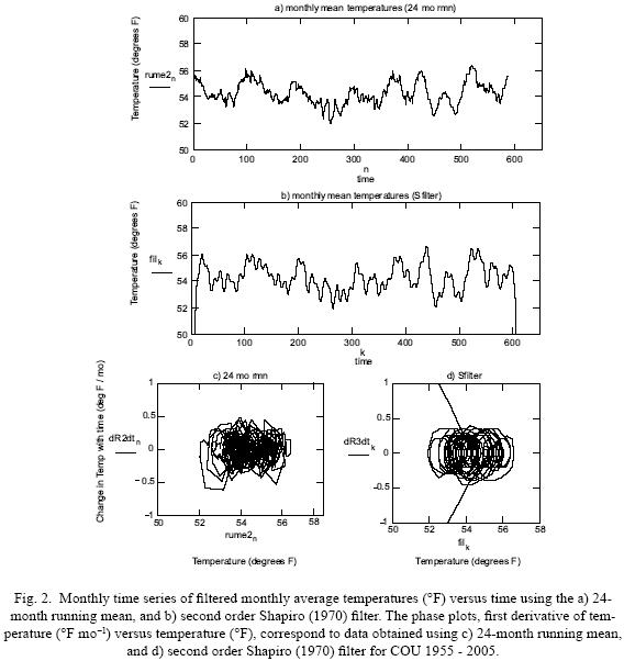
As in Mokhov et al. (2000, 2004), the goal here was to find periodicities on the interannual and interdecadal time–scale. Then, a filtering procedure was applied to the time series in order to extract this low order variability, or oscillations on a time–scale longer than two–years. Mokhov et al. (2000, 2004) presented results using a two–year running mean. The use of a two year running mean either requires having two additional years' worth of data than the analysis period, or the loss of two years worth of information. Here we use a simple second–order Shapiro (1970) filter applied repeatedly (here 60 times) to extract low order variability. In its simplest form, the filter is a three–point, center point–weighted stencil that is constructed based on the algorithm outlined by Shapiro (1970). The advantage to using this filter is that, with the exception of the two end–points, the length of the time series is retained, and the filter can be applied a successive number of times in order to effectively control the retention of signal versus noise. Due also to the symmetrical nature of this filter, it still preserves some of the annual cycle, does not result in a phase–shift of the low–order variability, and does not introduce significant aliasing error. A simple running mean filter may not necessarily possess these same characteristics (Shapiro, 1970). The Shapiro (1970) filter has been used effectively in other published studies to filter data fields in space for dynamic analyses of atmospheric blocking events in order to preserve their local character (Lupo, 1997; Lupo and Smith, 1998).
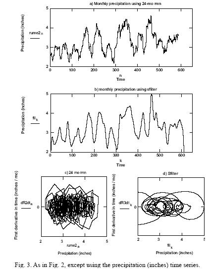
A comparison of the filtered temperatures (Fig. 2a, b) using each technique demonstrates that each captures the main features of the longer term variability. The phase plots produced by the 2–year running mean (Fig. 2c, d) also yield similar results, except that the phase plot produced using the Shapiro filter results in smoother trajectories (Fig. 2d). This results in a smoother analysis as the phase plot using the running mean filter (Fig. 2c) is difficult to analyze and may only suggest that the trajectories derived from temperature record over the time period is unstable (Zdunkowski and Bott, 2003) and/or the mean state was moving over time. However, the smoother phase plot using the Shapiro filter suggests that there were periods of time during the 1955–2003 record where the trajectories imply the monthly mean temperature record was stable (behaves like a damped oscillator), and there are periods of time when the record was unstable. Then, the system behaves similar to that suggested by Fedorov et al. (2003) who examined Pacific Region SSTs, and they suggest that the ENSO phenomenon behaved like a slightly damped oscillator, but was sustained by modest disturbances. This suggests that there are times in which the long–range monthly temperatures may be more predictable, instead of assuming that the system is solely chaotic or unpredictable at this time–scale. The same comparisons can be made using the precipitation records (Fig. 3).
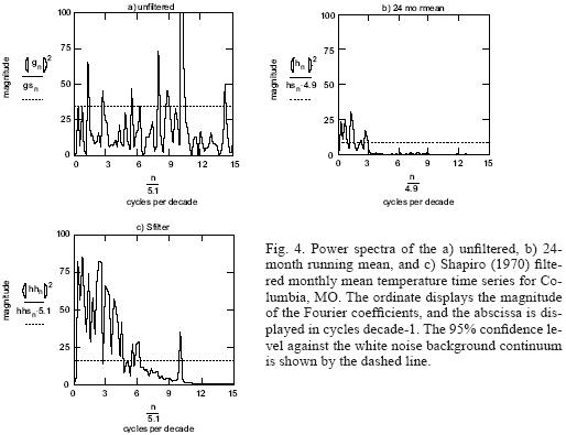
An examination of the temperature power spectra (Fig. 4) shows that the temperature series filtered, using the Shapiro filter (Fig. 4c), retains more power in the lower frequency oscillations than does the series filtered using the two year running means as a filter (Fig. 4b) producing a more robust signal at these lower frequencies. The power spectrum of the unfiltered temperature series is shown in Figure 4a for comparison, although for Figure 4b and c, the mean was removed before the FFT was applied. The annual cycle can easily be seen in this figure. Figure 4c also demonstrates that some of the annual cycle is still retained in the filtered temperature record. Figure 4c also demonstrates significant variability at about the 3, 6, and 20 year time periods, which is consistent with ENSO and interdecadal variability. The precipitation power spectra (Fig. 5) shows a similar result, however, the annual cycle is almost completely removed since the annual cycle is weaker in the precipitation time series. There are significant peaks at approximately the 3, 6, and 20 year time periods, and this analysis is consistent with that of Hu et al. (1998), who also analyzed Midwestern precipitation records using wavelet techniques and is also suggested by the use of proxy data (Guyette et al., 2002; Fye et al., 2003; Guyette and Stambaugh, 2003; Stambaugh and Guyette, 2004).

2.3 SST analysis
For each month, visual inspection of the monthly global SST and 500 hPa height charts was shown to be a reliable method for classifying the SST anomaly distributions into one of seven different synoptic categories (A–G) as defined in KC95 over the entire map area (Fig. 6). In order to be certain that this method was reliable, visual inspections of two years worth of monthly mean SST anomalies for randomly chosen months, within the period of study of KC95, were carried out in order to verify that observations of this group matched those of KC95. All months inspected by our group matched those of the KC95 study. Visual inspection was also used by KC95 after they used the clustering method of Fukunaga (1972) to derive their set of seven distinct anomaly types. They found that manual inspection yielded acceptable results. Methodologies in which manual analysis can be done quickly and easily would be useful in an operational forecasting environment.
3. Results of SST analyses
In Figure 6, examples of the seven different SST anomaly clusters are shown. These monthly global SSTs are not the same plots shown in KC95. Their plots represent the extracted large–scale mode, while here we show the actual monthly mean SSTs, which were classified similarly to those found in their Figure 1 over the entire map region. Thus, it is conceded that Figure 6 may contain smaller–scale noise. The characteristics of each type of anomaly are described in their paper, and the accompanying tropospheric height anomalies are also shown and described in their paper. Additionally, Enfield and Mestas–Nuñez (1999) and Mestas–Nuñez and Enfield (1999, 2001) performed a similar analysis on Pacific region SSTs and tropospheric variables. Since their analysis used a much longer time period, however, they were able to filter out multidecadal modes. Nonetheless, they found similar SST anomaly patterns to KC95. For example, Figure 1 from Mestas–Nuñez and Enfield (2001) is similar to the C cluster in KC95 (Fig. 1) and Figure 6c here. Given that there are some differences between these later studies and KC95, the discussion below is confined to KC95.
Briefly, SST clusters B and G are representative of La Niña type clusters in the Pacific Ocean basin. These are also characteristic of SST anomaly distributions in the Atlantic Ocean basin which are the opposite of each other. Clusters A and E are characteristic of ENSO neutral type conditions, including a fairly weak signal in the tropics and a stronger mid–latitude signal. These SST anomaly distributions are similar in each major ocean basin, with the exception that E–type anomalies are associated with a more widespread coverage of warm anomalies in general. The remaining clusters are C, D, and F type anomalies, which are representative of El Niño–type SST distributions in the Pacific Ocean basin. The D–type cluster represents fairly weak ENSO conditions, with the main SST anomaly located closer to the east–central Tropical Pacific. The C and F type anomalies represent stronger El Niño conditions, with the warm SST anomalies located in the far eastern Tropical Pacific Ocean. That the stronger ENSO events are associated with stronger SST anomalies located farther east agrees with the results of Clarke and Li (1995). C and F type anomalies are also similar to each other, with the exception that F type anomalies are associated with more widespread coverage of warm anomalies especially in the North Pacific and Atlantic Ocean basins. The C–type anomalies are characterized also by a strong warm SST anomaly oriented along the equator.
Table I was reproduced from KC95 (1955–1993) and then extended here from January 1994 through December 2005, and these results show that following 1993 there was an extended period of E–type anomalies (34 months, second longest period in the record), which correspond to the extended period of ENSO neutral conditions during the mid–1990s (Table II). This compares to the extended period (40 months, longest period in the record) of B–type anomalies which were characterized by La Niña and ENSO neutral conditions during the mid–1970s. This extended period of B–type anomalies was book ended by mostly C–type anomalies representing the 1972 and 1976 El Niños.
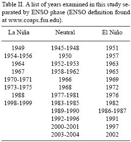
The strong El Niño of 1997 was characterized by the presence of F–type anomalies, and this El Niño was similar in character to the strong El Niño events of 1982 and 1986–1987. These El Niño events were also predominated by F–type SST anomalies, although a few C–type anomalies were associated with the 1982 El Niño. Thus, all the El Niño events that occurred during the period 1977–1998 were characterized by the presence of primarily F–type anomalies. This contrasts with the earlier period (1955–1976) when El Niño events were dominated by C and D–type anomalies (Tables I, II). Additionally, the beginning and end of each El Niño (Table I) described here was matched to the beginning and end as stated by the definition described in section 2. Each ended within one month of the end as identified by the JMA and each began within 2–4 months of the identified beginning using JMA. However, a perfect match would be difficult to obtain since, as described above, each month was classified by examining the global ocean SST distributions.
Then, during the latter part of 1998 through early 2002, the occurrence of G–type anomalies was prominent, but these were interspersed with the occasional periods of A, B or D type anomalies. The occurrence of G–type anomalies accompanied the La Niña years of 1998 and 1999 and becoming A and B type anomalies thereafter. Until the recent re–emergence of these G–type anomalies, this SST type was not observed to occur often in the KC95 analysis. In their analysis, these G–type anomalies were associated with La Niña years.
4. Further analysis of a local long–term temperature and precipitation time series
Park and Kung (1988) and Lee and Kung (2000) demonstrate that tropical Pacific SSTs have a significant influence on seasonal temperatures and precipitation variations and anomalies in the middle Mississippi region, and this information can then be used to make seasonal forecasts. They also demonstrate that there is approximately a 3–6 month lag between the tropical Pacific region SSTs and the seasonal climate of the middle Mississippi Valley region. These support the results of other studies which examined the impact of tropical SSTs on North American seasonal climates (Namias, 1982, 1983; Nakamura et al., 1997; Hu et al., 1998; Lupo and Bosart, 1999; Enfield and Mestas–Nuñez, 1999; Mestas–Nuñez and Enfield, 1999, 2001; Ratley et al., 2002). We note here however, that there is considerable disagreement among these and other studies about the degree of the impact of SSTs on mid–latitude weather and climate, and correlations between SSTs and climate do not describe any dynamic link between the two. Additionally, Hu et al. (1998), Ratley et al. (2002), and Palecki and Leathers (2000), who used principal component analysis, suggested that the interannual variability of temperatures and precipitation may behave similarly for most stations within this geographic region. Thus, the time series analyzed in section 2 will be analyzed further here and will serve as a sample for the mid–Mississippi valley region only.
The analysis in section 2b together with that in section 3 suggests that there is interannual and interdecadal variability in the time series for the Columbia monthly mean temperature and precipitation time series that is at least partially associated with ENSO and the PDO. Even though the analysis in 2b suggests that ENSO and PDO are cyclical, we recognize that these cycles are quasi–periodic and this may explain partially the imperfect correspondence cited in the previous sentence. In this section, we are also not necessarily interested in the change in the amplitude and frequency of ENSO on an interdecadal time–scale as shown by others in both observational (Gu and Philander, 1995; Mokhov et al., 2000) and model (Mokhov et al., 2004) studies. The goal of this section is to determine if specific climate regimes for this area can be associated with the SST types shown in section 3. However, these associations cannot discriminate the cause and effect of these linkages. Additionally, a detailed analysis of the relationship of conditions for particular seasons with each cluster will be the subject of a follow up study.
Hu et al. (1998) and Changnon (2003) identify interdecadal variability in mid–Mississippi regional precipitation time series and historical records (Fye et al., 2003), and the Hu et al. (1998) study attributed these to interdecadal modes in the North Atlantic Oscillation (NAO). This study suggests that the interdecadal variability in the region would more naturally be associated directly with PDO modes (as the mid–Mississippi Valley is downstream of the Pacific Region), and that SST distributions associated with the PDO modes would modulate those associated with the ENSO, and thus manifest itself in interdecadal variations in ENSO variability (Gershunov and Barnett, 1998).
That we attribute interdecadal variability here to PDO modes does not necessarily contradict the results of Hu et al. (1998), as other studies have identified a relationship between the PDO and NAO through the deep ocean global circulations (Gray, 1998; Houghton et al., 2001).
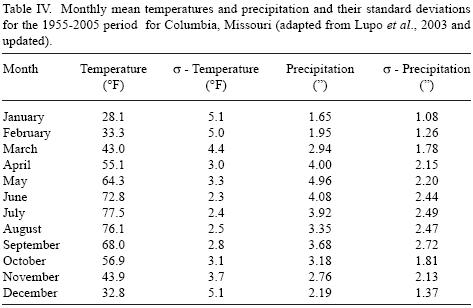
Then, in order to evaluate whether, for example, one type of SST anomaly (Table I) can be associated with a particular temperature and precipitation regime, only persistent periods (greater than four consecutive months) of one type of SST patterns were examined. There may be periods of time when the monthly temperature and precipitation regime may be more predicable in this region (as suggested by Figs. 2 and 3) even though, in general, the current state of forecasting the onset or demise of the ENSO–related SSTs is poor (Federov et al., 2003). This also insures that a particular type of anomaly is persistent for at least one season. Further, in order to account for a lag period in the large–scale circulations, as identified by previous authors referenced in section 1 between SSTs and North American climates, the first 3 months of a persistent SST regime were excluded from the analyses. In spite of these strict criterion, over half the months in the entire 1955–2005 series were included in association with one of the seven SST regimes in a persistent episode (331 out of 612). Each month's temperature and precipitation anomalies were calculated and then compared to the 1955–2005 mean values and standard deviation for that individual month (Table IV). This analysis then assumed a normal distribution for each parameter, which is a good assumption for this region (see Lupo et al., 2003), and months in which the anomaly was greater than one standard deviation higher or lower than the mean was considered an unusual occurrence.
The results of this analysis are shown in Figure 7 and Table V. In Figure 7, the probability distributions are displayed using a bar–graph. A normal distribution would appear as given by the key. None of temperature and precipitation regimes associated with each SST type could be classified as a normal distribution at standard levels of confidence (90% or more), when tested using a simple chi–square goodness–of–fit test and assuming the null–hypothesis or that there is no a priori relationship between SSTtype and temperature regime. Table V demonstrates that most of the SST regimes produced sufficiently large samples, with only the C and G–type SST regime resulting in fewer than 30 members. It is also conceded a posteriori that, due to shorter term oscillations (e.g., the 30–60 day oscillation) in the observations, statistical relationships may be difficult to establish in the raw data. We attempt, nonetheless, to find useful relationships based on the raw data as such information is routinely archived and analyzed most frequently in an operational sense.
4.1 PDO2 SST clusters
As shown in section 3, the predominant SST modes during the PDO2 years were of types A–D. Of these type, prolonged periods of A, B, D and G–type anomalies were nearly exclusive to these years. For the A–type regime, the distribution monthly mean temperature regime was biased toward lower temperatures, but these departures did not rise to the level of statistical significance (Fig. 7a) at the 90% confidence level. The precipitation regime was also biased toward drier months being associated with A–SST types, and this distribution was different from that of anormal distribution at the 90% confidence level (Fig. 7b). When monthly anomalies were considered as covariate set (warm–wet, warm–dry, cool–wet and cool–dry, respectively), there were nearly equal numbers of months in each bin, with the exception that there were more cool–dry months (Table V). The analysis of prolonged B–type anomalies showed no biases in either the temperature or precipitation distribution that rose to the level of statistical significance (Fig. 7c, d). While the monthly mean temperatures were biased toward warmer months during B regimes, these months were evenly split between warm and wet, and warm and dry regimes. A simple test for the statistical independence of bi–variate multinomial populations (here monthly mean temperatures and precipitation) demonstrated that for the A and B–type regimes, these variables were independent of each other. In addition, the A and B type anomalies do not display very a strong tropical signal, but they do have a stronger extra tropical SST signal. Again, Kushnir et al. (2002) showed that extratropical anomalies are not as influential on extratropical weather and climate as natural synoptic variability. Thus, this may explain the weak correspondence between A and B patterns, and the climate of the mid–Mississippi Valley region.
An analysis of prolonged D–type regimes demonstrates that the monthly mean temperatures were slightly biased toward warmer months (Fig. 7g), and the distribution is different from the normal distribution at the 95% confidence interval indicating a strong relationship. Prolonged D–type regimes are heavily skewed toward the drier months (67% of these months were drier than normal) (Fig. 7h), and this distribution was characterized as different from normal at the 99% confidence level. However, the cooler than normal months were split nearly evenly between wet and dry months. Given the strong combination of warmer and drier months, when considering these as abivariate population, 45% of all D–type months (18) were warm and dry, and this relationship was significant at the 95% confidence level. This is particularly true of D–type months in the warm season (warm and dry), while D–type months tended to be evenly distributed between cooler and warmer than normal conditions for the region during the cold season. This was typified by comparing the prolonged D–type anomalies in 2002–2003 (2004–2005), in which four of six (all seven) months were cooler (warmer) than normal. In both cases, however, the period was drier than normal (10 of the 13 months).
A similar analysis for G–type anomalies reveals that both the monthly mean temperature and precipitation anomaly distributions (Fig. 7m, n) were different from normal at the 99% confidence level. The temperature (precipitation) regime was skewed toward warmer (wetter) than normal months. However, warmer than normal months were evenly distributed between wetter and drier than normal, while more than one third of all G–type months (12) were cool and dry. Warm season G–type months tended to be cool and dry, while cool season G–type months tended to be warmer than normal. When applying the same test for statistical independence of monthly mean temperature and precipitation in the D and G type regimes, these variables were found to be dependent variables at the 95% confidence level. That these variables demonstrate a high degree of statistical dependence in the D and G–type regimes, when there is no reason to believe that they should be dependent a priori, suggests that there may be synoptic patterns that are associated with D and G patterns, and this issue will be explored further in subsequent work. This also suggests that there is operational value for the results found here. Also, further testing found that there was no statistically significant correlation between the size and sign of these anomalies in spite of the statistical dependence.
4.2 PDO1 SST clusters
These years were dominated by the occurrence of more El Niño events and these were stronger (e.g., 1982–1983, and the 1997–1998 events). Prolonged periods of E or F type anomalies did not result in any associated statistically significant deviations in the temperature or precipitation distributions (Fig. 7i–l) independent of seasons. When considering the combined E and F categories, cool dry months accounted for more than one–third of all months, while the rest of the sample months were distributed evenly among each category. Among F–type months only (stronger El Niño–type), however, these tended to be cooler than normal during the summer months and much warmer than normal during the winter months. It is well known that there is a strong correlation (e.g., use the statistical tool found at http://www.cdc.noaa.gov/USclimate/Correlation supporting the observation that El Niño winters were warmer than normal in the Midwest and upper Midwest during the 1977–1998 period (when F anomalies were a dominant El Niño type during these winters). For E–type months only there was no distinct tendency for warm or cool season months and again the E–type SST pattern was representative of ENSO neutral or weak La Niña type conditions. The test for statistical independence of monthly mean temperatures and precipitation yielded similar results to the A and B–type regimes, in that temperature and precipitation were found to be independent variables in these regimes. Also, the explanation for the weak correspondence found for the E–category may also be similar to that for the A and B type anomalies.
4.3 C–type SST clusters
The sample size for prolonged C–type (ENSO type) clusters was small, but analyzing these is also more complex as it was the only SST type in which there were nearly equal occurrences of these in both PDO1 and PDO2 years. The overall behavior of these distributions (Fig. 7e, f) demonstrates that these distributions were different from normal, at the 95% confidence level for monthly mean temperatures and at 99% for precipitation. These C–type months were biased toward cooler conditions and wetter conditions, but temperature and precipitation were fairly evenly distributed when considering these as a bivariate population.
4.4 An initial seasonal analysis
Table VI displays the number of months in which the temperature and precipitation was above or below normal for the prolonged SST clusters analyzed above, in order to determine if particular seasons showed any bias toward particular conditions. No statistical analysis was performed here as the sample sizes are small. A follow–up study including larger samples is underway.
The warm bias noted in section 4.1 for the B–type clusters occurred primarily in the transition seasons, and these tended to be distributed such that the cold season as a whole was associated with warmer prolonged B–regimes. The dry bias found for the D–type clusters was nearly spread evenly throughout the year. In section 4.2, the cool bias found in association with E and F–type anomalies was evenly distributed throughout the year, with the exception of winter season F–type anomalies. These months were associated with warmer than normal conditions and half of these warm anomalies were one to two standard deviations above the normal for the winter months. Finally, the cool biases associated with the C–type clusters were especially strong during the June–February period, which resulted in cooler condition during the first part of the cool seasons.
5. Summary and conclusions
Using monthly mean global SST and 500 hPa height data routinely available via the Internet or regular monthly publications, as well as monthly mean temperature and precipitation time series from 1955–2005 for a station that is representative of the mid–Mississippi valley, interannual and interdecadal variations in the climate of this region were examined. In performing an analysis on the time series to identify the predominant low–order modes, even though ENSO and PDO are quasi–periodic, the techniques of Mokhov et al. (2004) (and references therein) were demonstrated and used with a beneficial modification of the filtering technique presented here. This modification resulted in smoother analysis of the phase plot without degrading the ability of Fourier or wavelet techniques to identify the predominant long–term modes.
The SST anomaly classification archive initiated by KC95 for the period 1955–1993 was updated to include all months through the end of 2005. Visual inspection of the SST anomalies and selected 500 hPa height anomalies were performed successfully, in order to verify that this analysis agreed with those of KC95. Then the months from January 1994 to December 2005 were examined and classified. An analysis was performed to determine whether there was a correlation between monthly SST anomalies, for each cluster and mid–Mississippi Region monthly temperature and precipitation anomalies.
The results validate the conclusions of KC95, in that SST clusters B and G (C, D, F) [A and E] are representative of La Niña (El Niño) [neutral] conditions within the Pacific Ocean basin. In particular, the period 1955–1976 was dominated by SST types A–D, while the period 1977–1998 was associated with the occurrence of E, F, and occasionally C modes. In the most recent period G, A and B modes have predominated. Finally, the most recent months have marked the occurrence of weak El Niño events (2002–2003, 2004–2005), which were associated with D–type anomalies. Thus, these most recent El Niño events were closer in character when examining just the SSTs to El Niño events of the 1955–1976 period rather than the El Niño events of the 1977–1998, in that they were predominantly D type clusters (Table I)
A further examination of the monthly mean temperature and precipitation records showed that the long–lived SST clusters were not associated with normally distributed monthly temperature and precipitation anomalies, unlike those of the total 51 year period for the mid–Mississippi region (Lupo et al., 2003). However, neither were most of the long–lived SST clusters associated with statistically significant deviations from that of normal. Only the long–lived D– (G–) type clusters were associated with distributions skewed toward warmer and drier (wetter) conditions, and these were associated with El Niño– (La Nina–) years. However, during D– (G–) type months the statistical analysis of these two flow regimes was not straightforward, since during these months the most common occurrence when treating the data as a bivariate population were warm and dry (cool and dry) months. The statistical test for independence demonstrated a statistical dependence between temperature and precipitation anomalies in these regimes, which may be explained by further examination of the 500 hPa height anomaly distributions. Work is continuing in this area. Additionally, a correlation between the strength of monthly temperature and precipitation anomalies for each of these regimes did not rise to the level of statistical significance.
A study of prolonged SST anomalies stratified by type could be the subject of future work when a greater volume of reliable data becomes available. Finally, it may not be enough to examine interannual variability over a consecutive 50, 70, or even 100 year period since the occurrence and amplitude of the ENSO phenomenon may change over an extended period (Gu and Philander, 1995; Mokhov et al., 2004), and thus result in a changed or modulated ENSO response in local climatic parameters of an interdecadal time–scale (Gershanov and Barnett, 1998; Lupo et al., 2003). Nonetheless, this work has provided useful information for long–range forecasting guidance for temperatures and precipitation in the mid–Mississippi valley.
Acknowledgements
The authors would like to thank Dr. Ernest C. Kung for his contribution in discussing some of these results. We also thank Mr. David Barriopedro–Cepero for his help in translating the abstract into Spanish. Finally, we would like to thank the two anonymous reviewers for their time and effort in making this manuscript a stronger contribution to the literature.
References
Anderson J., H. van den Dool, A. Barnston, W. Chen, W. Stern and J. Ploshay, 1999. Present–day capabilities of numerical and statistical models for atmospheric extratropical seasonal simulation and prediction. Bull. Amer. Meteor. Soc. 80, 1349–1362. [ Links ]
Arpe K., L. Bengtsson, G. S. Golitsyn, I. I. Mokhov, V. A. Semenov and P. V. Sporyshev, 2000. Connection between Caspian Sea level variability and ENSO. Geophys. Res. Lett. 27, 2693–2696. [ Links ]
Barnston A. G., H. van den Dool, S. E. Zebiak, T. P. Barnett, M. Ji, D. R. Rodenhuis, M. A. Cane, A. Leetmaa, N. E. Graham, C. R. Ropelewski, V. E. Kousky, E. A. O'Lenic and R. E. Livezey, 1994. Long–lead seasonal forecasts. Where do we stand? Bull. Amer. Meteor. Soc. 75, 2097–2114. [ Links ]
Berger C. L., A. R. Lupo, P. Browning, M. Bodner, C. C. Rayburn and M. D. Chambers, 2003. A climatology of northwest Missouri snowfall events: Long term trends and interannual variability. Phys. Geog. 23, 427–448. [ Links ]
Changnon S. A., 2003. Temporal distribution of midwestern precipitation during the 20th Century. Illinois, State Water Survey Tech. Doc. 2003–01, 32 pp. [ Links ]
Clarke A. J. andB. Li, 1995. On the timing ofwarm and cold El Niño–Southern Oscillation Events. J. Climate. 10,2571–2574. [ Links ]
Enfield D. B. and A. M. Mestas–Nuñez, 1999. Multiscale variabilities in global sea surface temperatures and their relationships with tropospheric climate patterns. J. Clim. 12, 2719–2733. [ Links ]
Federov A. V., S. L. Harper, S. G. Philander, B. Winter, and W. Wittenberg, 2003. How predictable is El Niño? Bull. Amer. Meteor. Soc. 84, 911–920. [ Links ]
Fukunaga K., 1972. Introduction to statistical pattern recognition. Academic Press, New York, 369 pp. [ Links ]
Fye F. K., D. W. Stahle and E. R. Cook, 2003. Paleoclimatic analogs to twentieth Century moisture regimes across the United States. Bull. Amer. Meteor. Soc. 84, 901–910. [ Links ]
Gershunov A. and T. P. Barnett, 1998. Interdecadal modulation of ENSO teleconnections. Bull. Amer. Meteor. Soc. 79, 2715–2725. [ Links ]
Gray W. M., 1998. Hypothesis on the cause of global multidecadal climate change. Preprints of the Ninth Symposium on Global Change Studies, 11–16 January, Phoenix, AZ, 271–275. [ Links ]
Gray W. M., J. D. Sheaffer, and J. A. Knaff, 1992. Influence of the stratospheric QBO on ENSO variability. J. Meteor. Soc. Japan 70, 975–995. [ Links ]
Gray W. M., 1984. Atlantic season hurricane frequency. Part 1: El Niño and 30 mb quasi biennial oscillation influences. Mon. Wea. Rev. 112, 1649–1668. [ Links ]
Gu D. and S. G. H. Philander, 1995. Secular changes of annual and interannual variability in the tropics during the past century. J. Climate 8, 864–876. [ Links ]
Guyette R. P. and M. C. Stambaugh, 2003. The age and density of ancient oak in streams and sediments. International Association of Wood Anatomists J. 24, 345 – 353. [ Links ]
Guyette R. P., W. G. Cole, C. D. Dey and R. M. Muzika, 2002. Perspectives on the age and distribution of large wood in riparian carbon pools. Canad. J. Fish. Aqu. Sci. 59, 578 – 585. [ Links ]
Hoskins B. J., I. N. James and G. H. White, 1983. The shape, propagation, and mean–flow interaction of large–scale weather systems. J. Atmos. Sci. 40, 1595–1612. [ Links ]
Houghton J. T., Y. Ding, D. J. Griggs, M. Noguer, P. J. van der Linden and D. Xiaosu, 2001. Climate change 2001: The scientific basis. Cambridge University Press, Cambridge, UK, 857 pp. [ Links ]
Hu Q., C. M. Woodruff, and S. E. Mudrick, 1998. Interdecadal variations of annual precipitation in the Central United States. Bull. Amer. Met. Soc. 79, 221–230. [ Links ]
Kalnay E., M. Kanamitsu, R. Kistler, W. Collins, D. Deaven, L. Gandin, M. Iredell, S. Sha, G. White, J. Woolen, Y. Zhu, L. Chelliah, W. Ebisuzaki, W. Higgins, J. Janowiak, K. C. Mo, C. [ Links ]
Ropelewski, J. Wang, A. Leetmaa, R. Reynolds, R. Jenne and D. Joseph, 1996. The NCEP/NCAR40–year reanalysis project. Bull. Amer. Meteor. Soc. 77, 437–471. [ Links ]
Keables M. J., 1992. Spatial variability of the mid–tropospheric circulation patterns and associated surface climate in the United States during ENSO winters. Phys. Geog. 13, 331–348. [ Links ]
Kerr R. A., 1999. Big El Niños ride the back of slower climate change. Science 283, 1108–1109. [ Links ]
Key J. R. and A. C. K. Chan, 1999. Multidecadal global and regional trends in 1000 mb and 500 mb cyclone frequencies. Geophys. Res. Lett. 26, 2053–2056. [ Links ]
Kousky V. E, G. D. Bell, M. S. Halpert and W. Higgins (Eds.) 2002. Climate Diagnostics Bulletin. A monthly publication of the Climate Prediction Center. Camp Springs, MD, USA, 92 pp. [ Links ]
Kung E. C. and J.–G. Chern, 1995. Prevailing anomaly patterns of the global sea surface temperatures and tropospheric responses. Atmósfera 8, 99–114. [ Links ]
Kunkel K. E. and J. R. Angel, 1999. Relationship of ENSO to snowfall and related cyclone activity in the contiguous United States. J. Geophys. Res. 104, 19425–19434. [ Links ]
KushnirY., W. A. Robinson, I. Bladé, N. M. J. Hall, S. Peng and R. Sutton, 2002. Atmospheric GCM response to extratropical SST anomalies: Synthesis and evaluation. J. Clim. 15, 2233–2256. [ Links ]
Lee J.–W. and E. C. Kung, 2000. Seasonal–range forecasting of the Ozark climate by a principal component regression scheme with antecedent sea surface temperatures and upper air conditions. Atmósfera 13, 223–244. [ Links ]
Lorenz E. N., 1963. Deterministic nonperiodic flow. J. Atmos. Sci. 20, 130–141. [ Links ]
Lupo A. R., E. P. Kelsey, E. A. McCoy, C. E. Halcomb, E. Aldrich, S. N. Allen, F. A. Akyuz, S. Skellenger, D. G. Bieger, E. Wise, D. Schmidt, and M. Edwards, 2003. The presentation of temperature information in television broadcasts: What is normal? Nat. Wea. Dig. 27, 53–58. [ Links ]
Lupo A. R. and G. Johnston, 2000. The interannual variability of Atlantic Ocean basin hurricane occurrence and intensity. Nat. Wea. Dig. 24, 1–11. [ Links ]
Lupo A. R., and L. F. Bosart, 1999. An analysis of a relatively rare case of continental blocking. Quart. J. Roy. Meteor. Soc. 125, 107–138. [ Links ]
Lupo A. R. and P. J. Smith 1998. The interactions between a mid–latitude blocking anticyclone and synoptic–scale cyclones occurring during the Northern Hemisphere summer season. Mon. Wea. Rev. 126,503–515. [ Links ]
Lupo A. R. 1997. A diagnosis of two blocking events that occurred simultaneously in the mid–latitude Northern Hemisphere. Mon. Wea. Rev. 125, 1801–1823. [ Links ]
Lupo A. R., P. J. Smith, and P. Zwack, 1992. A diagnosis of the explosive development of two extratropical cyclones. Mon. Wea. Rev. 120, 1490–1523. [ Links ]
Mantua N. J., S. R. Hare, Y. Zhang, J. M. Wallace and R. C. Francis, 1997. A Pacific interdecadal climate oscillation with impacts on salmon production. Bull. Amer. Meteor. Soc. 78, 1069–1079. [ Links ]
Mestas–Nuñez A. M. and D. B. Enfield, 2001. Eastern equatorial Pacific SST variability: ENSO and non–ENSO components and their climatic associations. J. Climate 14, 391–402. [ Links ]
Mestas–Nuñez A. M. and D. B. Enfield, 1999. Rotated global modes of non–ENSO sea surface temperature variability. J. Climate 12, 2734–2746. [ Links ]
Minobe S., 1997. A 50–70 year climatic oscillation over the North Pacific and North America. Geophys. Res. Lett. 24, 683–686. [ Links ]
Mokhov I. I., 1995. Diagnostics of climatic system structure and its evolution in the annual cycle and interannual variability. Moscow, IAP RAS, 64 pp. (In Russian) [ Links ]
Mokhov I. I. and A. V. Eliseev, 1998. Tendencies of change of QBO characteristics for zonal wind and temperature of equatorial lower stratosphere. Izvestiya, Atmos. Ocean. Phys. 34, 327–336. [ Links ]
Mokhov I. I., D. V. Khvorostyanov and A. V. Eliseev, 2004. Decadal and longer–term changes in ENSO characteristics. I. J. Climatol. 24, 401–414. [ Links ]
Mokhov I. I., A. V. Eliseev and D. V. Khvorostyanov, 2000. Evolution of characteristics of the climate variability related to the El Niño / La Niña phenomena. Izvestiya, Atmos. Ocean. Phys. 36,741–751. [ Links ]
Mokhov I. I., V. A. Bezverkhny and A. V. Eliseev, 1997. Quasi–biennial oscillations of the atmospheric temperature regime: Tendencies of change. Izvestiya, Atmos. Ocean. Phys. 33, 533–541. [ Links ]
Nakamura H., G. Lin and T. Yamagata, 1997. Decadal climate variability in the Northern Pacific during recent decades. Bull. Amer. Met. Soc., 78, 2215–2226. [ Links ]
NamiasJ., 1982. Anatomy of great plains protracted heat waves (especially the 1980 U.S. Summer drought). Mon. Wea. Rev. 110, 824–838. [ Links ]
Namias J.,1983. Some causes of the United States drought. J. Clim. Appl. Met., 22, 30–39. [ Links ]
Palecki M. A. and D. J. Leathers, 2000. Spatial modes of drought in the central United States. Preprints of the 12th Conference on Applied Climatology, 8–11 May, Asheville, NC. [ Links ]
Park C.–K. and E. C. Kung, 1988. Principal components of the North American summer temperature field and the antecedent oceanic and atmospheric condition. J. Meteor. Soc. Japan 66, 677–690. [ Links ]
Peixoto J. P. and A. H. Oort, 1992. The physics of climate. American Institute of Physics, New York, 520 pp. [ Links ]
Quiroz R. S., 1984. The climate of the 1983–1984 winter – a season of strong blocking and severe cold over North America. Mon. Wea. Rev. 112, 1894–1912. [ Links ]
Ratley C. W., A. R. Lupo and M. A. Baxter, 2002. Determining the spring to summer transition in the Missouri Ozarks using synoptic–scale atmospheric data. Transactions of the Missouri Academy of Science 36, 69–77. [ Links ]
Renwick J. A. and M. J. Revell, 1999. Blocking over the south Pacific and Rossby wave propagation. Mon. Wea. Rev. 127, 2233–2247. [ Links ]
Shabbar, A., J. Huang, and K. Higuchi, 2001. The relationship between the wintertime North Atlantic Oscillation and blocking episodes in the North Atlantic. Int. J. Climatol. 21, 355–369. [ Links ]
Shapiro R., 1970. Smoothing, filtering, and boundary effects. Rev. Geophys. 8, 737–761. [ Links ]
Stambaugh M. C. and R. P. Guyette, 2004. Long–term growth and climate response of shortleaf pine. 14th Annual Central Hardwoods Conference Proceedings, Wooster OH, March 2004. USDA Forest Service, General Technical Report, GTR–NE–316. 448–458. [ Links ]
Vincent D. G., 1994. The south Pacific convergence zone (SPCZ): A review. Mon. Wea. Rev. 122, 1949–1970. [ Links ]
Wallace J. M. and D. S. Gutzler, 1981. Teleconnections in the geopotential height field during the northern hemisphere winter. Mon. Wea. Rev. 109, 784–812. [ Links ]
Wiedenmann J. M., A. R. Lupo, I. I. Mokhov and E. A. Tikhonova, 2002. The climatology of blocking anticyclones for the northern and southern hemisphere: Block intensity as a diagnostic. J. Climate 15, 3459–3474. [ Links ]
Zdunkowski W. and A. Bott, 2003. Dynamics of the atmosphere: A course in theoretical meteorology. Cambridge University Press, UK, 719 pp. [ Links ]

