Short contribution

 

Maximum ground level concentration of air pollutant

 

M. EMBABY, A. B. MAYHOUB, K. S. M. ESSA and S. ETMAN

Mathematics and Theoretical Physics Department, Nuclear Research Center, Atomic Energy Authority, Cairo, Egypt

 

(Manuscript received Feb. 15, 2001; accepted in final form Aug. 29, 2001)

 

RESUMEN

Por medio del modelo de pluma gaussiana, se obtiene la concentración superficial de un contaminante aéreo. Sin embargo, la altura efectiva H del contaminante se considera como función de las coordenadas superficiales x y y. Se desarrolla el radio extremo de la chimenea. La constancia de H se estudia como un caso especial del problema. Se deducen argumentos interesantes sobre las concentraciones máxima y peor.

 

ABSTRACT

The ground level concentration of an air pollutant is obtained using the Gaussian plume model. However, the effective height H of the pollutant has been considered as a function of the ground level coordinates x and y. Extreme radius of the stack is developed. The constancy of H has been studied as a special case for the problem. Interesting arguments about both maximum and worst concentrations have been derived.

Key words: Gaussian plume, stack, pollutant concentration.

 

1. Introduction

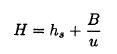
The Gaussian plume model (GPM) (Csanady, 1973; Smith, 1973; Turner, 1970) provided the primary method for calculation concentration of non-reactive pollutants from a point source. This model has found widespread application in design of stacks and environmental impact analysis. In the GPM formula for the concentration, the effective height for emission is an important parameter for ground level concentrations. Due to the initial kinetic energy of the released plume and its thermal energy when the plume temperature is above ambient air temperature, there will be an increase in the emission height of the plume. This increase is known as the plume rise Δh. The effective source height H is then given by:

Where h_s is the physical stack height. In order to predict ground level concentration of pollutants, the plume rise should be taken into consideration. Pasquill (1971); Ragland (1975) and others have obtained the maximum ground level concentration, taking into account a constant plume rise Δh with the downwind distance x. In this paper, we shall generalize the case for which Δh (and consequently, the effective source height H) is a function of ground level coordinates x. and y, i. e., H = H(x, y). The effective height H will be obtained in terms of x, and y. Power law forms of the dispersion coefficients σ_z and σ_y namely (Ragland, 1975):

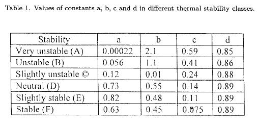
have been assumed through the treatment. The coefficient a, b, c, and d are real numbers depending on the atmospheric stability classes, as shown in Table (1) (Ragland, 1975).

 

2. Mathematical treatment

The concentration distribution from a single continuous point source at some point above the ground is given by the Gaussian plume model (IAEA, 1983) as:

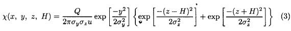
where

x - is the downwind distance from the source (m),

y - is the crosswind distance from the source (m),

z - is the vertical distance above the ground (m),

χ - is the concentration of pollutant (g/m³),

u - is the downwind velocity is taken along the x-axis (positive direction) (m/sec),

Q - is the source strength (g/sec),

H - is the effective stack height (m),

σ_y and σ_z are given by equation (2) are the standard deviations of plume concentration distribution in the horizontal and vertical directions respectively.

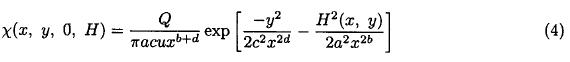
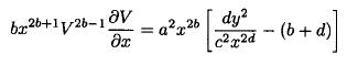
The ground level concentration is obtained by setting z = 0 in (3), and on substitution the values of σ_y and σ_z from (2) into (3), we get:

Maximum ground level concentration occurs when δχ/δx = 0 which gives

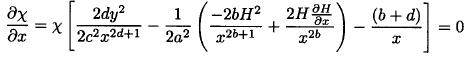
From which we get

Assuming the following substituting

Equation (5) is reduced to:

Which on integrating both sides with respect to x, gives:

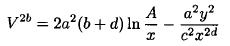
where A is a constant of integration. From equation (6), we can write:

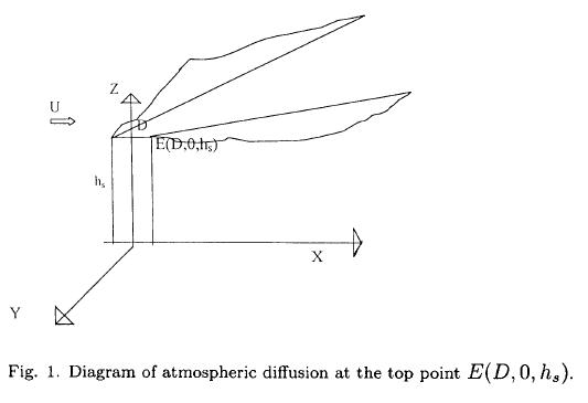
This equation represents a relation between the point (x, y) of the pollutant path and its corresponding height H. In order to deduce A we can satisfy equation (7) at certain point E(D, 0, h_s) on to top of the stack, where the air pollutant starts to move at velocity u along the x-direction, where D is the radius of the stack (Fig. 1). Substituting the coordinates of the point E into equation (7), we obtain the constant A in the form:

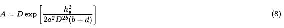
Substituting from (8) into equation (7), we get:

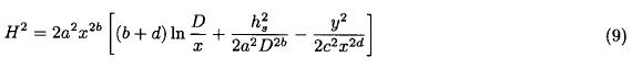
This equation describes the pollutant height H in terms of the position (x, y). Now, substituting from (9) into (4), we get the desired expression for the maximum ground level concentration in the form:

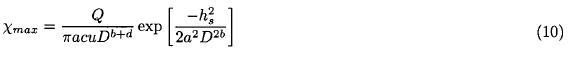
It is evident that the concentration χ_max depends on both meteorological parameters and release characteristics.

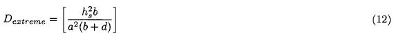
From (10) one can determine the extreme radius D for the stack that gives maximum ground level concentration. This can be obtained by differentiating χ_max partially with respect to D and let

Which implies:

Referring to equation (10), when differentiating with respect to h_s and let the result equals zero, we can verify the simple and realistic result that the higher stack the minimum the value of the concentration.

 

3. Special case

Now, we consider the case where the effective height H is constant, i. e. does not depend on x and y.

Since the air pollutant masses just in the wind velocity direction, i. e. along the x-axis where y = 0, the substitution of both y = 0 and δH/δx = 0 into equation (5) gives:

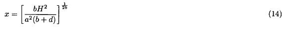
Hence, the point of maximum ground level concentration of the pollutant has the coordinates

That is lies on the x-axis.

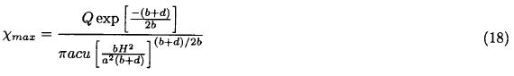
Now, substituting the values of x_max into equation (2) we obtain the maximum dispersion coefficient:

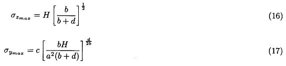
Then, the maximum ground level concentration χ_max could be easily identified using equation (4) and (15):

 

4. Worst ground level concentration

It is well known that the release height H is inversely proportional to the wind velocity, u, hence the plume rise Δ can be written in the form:

where B is a characteristic constant for every stability class and for a particular stack. To find the worst wind velocity u_worst under which, the ground level concentration has maximum value, we find dχ/du = 0. Differentiating equation (18), and taking into account that

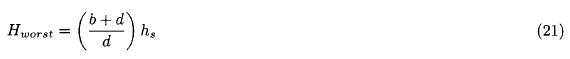
we get

From which, the worst emission height H_worst which causes a maximum ground level concentration is given by:

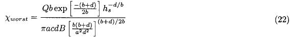
Finally, substituting u_worst and H_worst back into equation (18), we get the worst ground level concentration, namely:

 

5. Numerical study

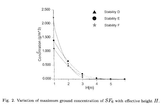
Now, let us consider some specific data (Start and Hoover, 1995) for Q = 9.4 g/sec, u = 4.1 m/sec, and D = 3 m for different stability classes, namely Neutral (D), Slightly stable (E), and Stable (F). Using Table (1) in combination of equation (10), we can obtain graphical relation between the maximum values for the ground level concentration of Sulferhexaflouride, SF₆ and its corresponding effective height. It is evident that such concentrations are inversely proportional to the effective height H as shown in Figure 2.

 

6. Summary and conclusions

A mathematical treatment has been proposed for the ground level concentration of a pollutant from a continuously-emitted point source. An analytic solution has been obtained in two cases: (1) The effective height H of the pollutant is a function of the ground level coordinates x and y, i. e., H = H (x, y), and (2) H is constant.

Extreme diameter of the stack has been taken into consideration. The position of maximum ground level concentration has been easily verified in the case of constancy of H. It was difficult to determine such position when H = H(x, y) because of the complexity of relation (9). The worst of both velocity and ground level concentration has been established in order to determine the velocity where maximum ground level concentration occurs. Numerical calculations were considered to realize the values of maximum concentration and its corresponding heights elevations in some different stability classes for SF₆.

 

REFERENCES

Csanady, G. T., 1973. Turbulent diffusion in the environment, Reidel, Dordrecht, Holland, 248 pp.         [ Links ]

IAEA safety guide, 1983, No. 50-SG-S3.         [ Links ]

Pasquill, F., 1971. Atmospheric dispersion of pollution, Q. J. R. Met. Soc., 97, 369.         [ Links ]

Ragland, K. W., 1975. Point source atmospheric diffusion model with variable wind and diffusivity profiles, Atmospheric Environmental, 9, 175.         [ Links ]

Ragland, K. W., 1975. Worst case ambient air concentration from point source using the Gaussian plume model. Atmospheric Environmental, 10, 371.         [ Links ]

Smith, M. E., 1973. Guide for the prediction of the dispersion of airborne effluent, ASME.         [ Links ]

Start, G. E. and D. Hoover, 1995. Model validation program. Cape Canaveral, Florida, Technical report, NOAA Air Resources Laboratory, Field Research Division, Idaho Falls, ID.         [ Links ]

Turner, D. B., 1970. Workbook of atmospheric dispersion estimates, U. S. Environmental Protection Agency Ap-26.         [ Links ]