


 nueva página del texto (beta)
 Inglés (pdf)
 Artículo en XML
 Referencias del artículo
 Enviar artículo por email
 Citado por SciELO
  Similares en
SciELO
Similares en
SciELO 
 Permalink
Introduction
According to Bingham (2013), working with financial series involves a series of challenges since financial series tend to show asymmetry, i.e., bias, leptokurtosis, and periods of high volatility resulting from the complex financial and economic environment. Therefore, sometimes an indicator is needed that helps the market participants to measure the volatility of the markets. In the case of the foreign exchange markets, the implied or realized volatility can be used for the foreign exchange or for a stock index. However, if one wants to calculate volatility in a fixed-income market which has more than fifty securities that also are highly correlated, the estimation of one number that measures the volatility is more complicated. The purpose of this paper is to develop a methodology for the estimation of the volatility of the fixed-income markets in Mexico that includes the analysis of zero-coupon bonds, fixed rate bonds, inflation-linked bonds and interest rate swaps. For the estimation of the volatility, a method is proposed based on Alexander (2001), who shows how orthogonal factors are used to simplify the process of variance-covariance matrix estimation.
There are several methods to estimate volatility in fixed income markets. The first is the volatility in the price. However, the price is affected by changes in the interest rates, the accrued interest, and the payment of coupons. The other two approaches are focused on the changes of the yield to maturity that is the internal rate of return of the asset. Fixed-income instruments trade in yield, which allows investors to know and compare the return of different assets independently of the maturity or size of the coupon. The variance of this yield could be estimated using the percentage change or a simple difference change. For this work, the approach of simple difference is used as it is consistent with interest rate models of volatility such as Vasicek and it is a common method used in research. Even if it is possible to estimate the variance and volatility of each asset, it is not possible to solve the problem of calculating the volatility of the yield curve, which is composed of all the fixed income assets of the same class in order from the asset with the lowest maturity to the asset with the highest maturity. As expected, there is an important correlation of the yields with maturity, in particular those that are adjacent. Then, in order to estimate the volatility of the curve using an approach similar to the Markowitz Mean-Variance optimal portfolio, it will be necessary to compute the variance-covariance matrix of the changes in the yield of the assets that belong to the yield curve.
Usually, the calculation of variances and covariances reusing the formulas for the covariance and variance historical or exponential moving averages, has not been very effective when estimating and predicting the volatility that the participants in the market currently face, and implies the estimation of n(n+1)/2 parameters. The general model of conditional autoregressive heteroscedasticity (GARCH) developed by Engle and Bollerslev has proved to be better than other models when estimating current volatility and forecasting volatility in the short-term, according to Alexandre (2001). Therefore, it is desirable to apply a GARCH model to estimate the volatility of the different yield curves in the Mexican financial market. However, the use of multivariate GARCH for more than two or three involves some difficulties due to the number of parameters that must be estimated and could involve problems regarding the optimization of the likelihood function.
Section II contains the literature review. In section III, the description of the data and an analysis of principal components were performed for four yield curves: zero-coupon bonds, nominal bonds (M-bonds), inflation-linked bonds (Udibonos) and TIIE interestrate swaps. In section IV, a GARCH(1,1) was adjusted. It was decided to use a GARCH(1,1) because this model tends to be a standard. With these estimations, and using the orthogonality of the variable, it is possible to obtain the square root to obtain the volatility of the yield curve or even that of all the fixed-income market.
In section V, using the estimates for the variance-covariance computed using the orthogonal GARCH and the eigenvectors, the original variance-covariance and correlation matrices can be approximated, and can be used to optimize a portfolio or to obtain a matrix that excludes idiosyncratic behavior of a security. Finally, section VI contains the conclusions.
Literature review
According to Alexander (1998), the most widely accepted approach to risk in financial markets is the volatility of the returns. This variable, in the case of the yield curve that it is possible to consider as a bond portfolio, depends on the variances and the covariances between the risk factors. In the case of a bond portfolio it is possible to identify the main sources of risk, following the results of Litterman (1991). This author analysed the common factors which affect the returns on the U.S. government bond yield curve, identifying that the first factor corresponds to the level or parallel shift movements, the second one is the slope of the curve, and the last one is the curvature or convexity of the yield curve.
The identification of the three main sources of volatility for the yield curve is possible because the financial markets tend to have a high degree of collinearity, as was highlighted by Alexander (2001). The principal component analysis makes it possible to extract the most important uncorrelated sources of variations. Through this analysis it is possible to measure independently the volatility presented in the changes in each of these actors, as mentioned by Alexandre (2000). With these three estimations is possible to obtain a good estimator for the variance covariance matrix for all the bonds in the yield curve. According to Alexandre (2000), this approach presents the advantage of generating a positive semi-definite matrix, capturing only the main variations and eliminating the noise caused by small effects. The estimations are more stable than the direct estimation of the matrix.
There are several methods to estimate the volatility of financial assets, such as the exponentially weighted moving average or the ARCH and GARCH models developed by Engle, which have been widely accepted in finance, especially the GARCH(1,1) which tends to adjust the volatility of financial asset returns well. However, the estimation of a multivariate GARCH as proposed by Engle and Kroner (1993) becomes more complex as the number of variables increases. To avoid the problem of complexity, the uses of uncorrelated factors makes it possible to estimate orthogonal GARCH for the volatility of each factor. The Orthogonal GARCH is the principal components method. In the context of a GARCH, the principal components were applied by Ding (1994) and Alexander and Chibumba (1996), among others.
It should be mentioned that a generalization of the orthogonal GARCH was applied with simulated and observed data in Van Der Weide (2002). The most relevant studies of the linear dependences among markets are through multivariate GARCHs. In a world of strong links between financial markets, the multivariate setting for the study of volatilities and correlations is natural. An excellent survey of these multivariate GARCH models is provided by Bauwens, Laurent, and Rombouts (2006). With respect to the multivariate models of volatility, for example that of the returns, they can be successfully modelled through a multivariate t-student dynamic correlations model; see, for example, Dube S. (2016). The forecasting of the correlations and variances is an important issue that can be analyzed. In the case of exchange rates of the Nigerian Naira, the orthogonal GARCH models represent a good enough choice; see Godknows, Isenah, and Olubusoye (2016).
Data and Principal Components Analysis
The rates for different government instruments are published by the Mexican Central Bank (Banco de Mexico) and the source for the Swaps of TIIE are provided by PIP (Proveedor Integral de Precios).
The idea of this section is to reduce the dimension of each yield curve and at the same time obtain variables that are linearly independent, which implies correlation equal to zero among them. In the case of yield curves, it is commonly mentioned in the literature that the first three principal components are identified (Litterman, 1991), and are enough to model the behavior of the yield curve. Branch (2004) mentions several empirical studies which suggest that the first component corresponds to the parallel displacement of the curve of rates, while the second component is related to the slope of the curve and in general shows opposite changes between short- and long-term rates. Finally, the third component represents the factor of the curvature of the yield curve, typically showing higher coefficients for rates close to one year and less for long terms of the curve. It is worth mentioning that the variance associated with the other main components decreases rapidly; usually the three first components explain more than 95% of the total variance.
Once the principal components are obtained, the problem is reduced to computing a diagonal variance-covariance matrix of dimension 3x3 and then it is possible to compute the variance of the yield curve with the matrix trace. The method of principal components (PCA) is a method of multivariate analysis that makes it possible to extract the most important linearly independent data sources. Applying the PCA method to n stationary time series, it is possible to obtain n stationary and orthogonal series called principal components. At the same time, this methodology makes it possible to know what percentage of the variance is explained by each component. In the following analysis four of the most important yield curves for the Mexican market were used. The data for the analysis correspond to the market information from October 2015 to November 2017 for the following yield curves:
Zero-coupon bonds (Cetes): These are the simplest kind of fixed-income securities. The Federal Government issues these securities every week for the Cetes with maturity of 28, 91, and 182 days, and every four weeks for the Cetes with maturity of 364 days. In order to have a time series for different constant maturities and taking into consideration the low liquidity of these assets, the following maturities intervals were used: 0-69, 70-100, 101-150, 151-200, 201-250, 251-300, and 301-364 days. Each interval represents the maturity in days of the Cetes that can be compared in order to have a reference rate for each interval in the case of some securities that did not have any operations on a particular day. The data are obtained from the weighted average rate traded by brokerage houses and published by Banco de México on its web site for these intervals.
Nominal Bonds (M-Bonds): This instrument is also issued by the Federal Government with maturities at inception of 3, 5, 10, 20, and 30 years. The yield to maturity of the bonds had the following maturities: December 2017, June 2018, December 2018, December 2019, June 2020, June 2021, June 2022, December 2023, December 2024, March 2026, June 2027, May 2029, May 2031, November 2034, November 2036, November 2038, and November 2042. The data were obtained from the Banco de México web site and the yield is the weighted average of the transactions that were performed through brokerage houses.
Inflation-Linked Bonds (Udibonos): This instrument is also issued by the Federal Government with maturities at inception of 3, 10 and 30 years. The yield to maturity of the Udibonos had the following maturities: December 2017, June 2019, December 2020, June 2022, December 2025, November 2035, November 2040, and November 2046. The data were obtained from the Banco de México web site and the yield is the weighted average of the transactions that were performed through brokerage houses.
TIIE Interest-Rate Swaps: these instruments are the most traded Mexican fixed-income assets and 80% of their volume was performed offshore. The underlying of the swaps is the non-collateralized interbank interest rate of 28 days published every day by Banco de México. These instruments allow the counterparties to change the 28-day TIIE floating rate for a fixed rate for the term of the swaps with interest payments every 28 days. The most traded terms are: three months, six months, nine months, one year, two years, three years, four years, five years, seven years, ten years, twelve years, fifteen years, twenty years, and thirty years. The information on these securities was obtained from Bloomberg. It is worth mentioning that the quotes of these instruments are abbreviated in the following way: “the number of payments x the term of reference rate.” In this case, 1 represents 28 days, then a quote on the brokers’ screens of “13 x 1” implies 13 payments of 28 days TIIE, which represents a maturity of 364 days or one year.
In order to perform the principal component analysis, the KPSS and the Augmented Dickey-Fuller tests were applied for each time series of the interest rate changes. In all the cases the series prove to be stationary (see Appendix III).
Thus, a total of 46 different instruments divided into 4 asset classes would require a multivariate GARCH of dimensions between seven to seventeen depending on the number of assets in each yield curve. Due to the computational complexities, the methodology of principal components is applied to reduce the dimensions that are needed and at the same time to make it possible to work with a few variables that are linearly independent. The orthogonality of the series is important in order to perform an orthogonal GARCH that uses this property to compute the variance of a set of variables.
Analyzing the changes in the different yield curves calculated by the simple difference and computing the correlation among nodes, high levels of correlation appear, in particular on those nodes which are closest.
In Figure 1, the range that the interest rate of zero-coupon bonds had during the period and the principal components for this curve can be observed. For the zero-coupon bonds high correlation is observed, and similar behavior explained by the close relation of these securities with movements in monetary policy.
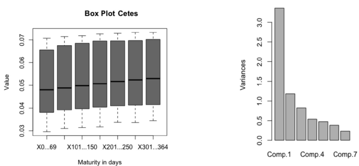
Source: own computations with Banco de Mexico Data.
Figure 1 Cetes Box-Plot and Principal Components
Figure 2 shows the range of the yield to maturity of the interest rates of nominal bonds during the period and their principal components.
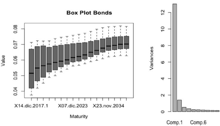
Source: own computations with Banco de Mexico Data.
Figure 2 Nominal Bonds (M-Bonds) Box-Plot and Principal Components
Figure 3 shows the range of the yield to maturity of the interest rates of inflation-linked bonds during the period and their principal components.
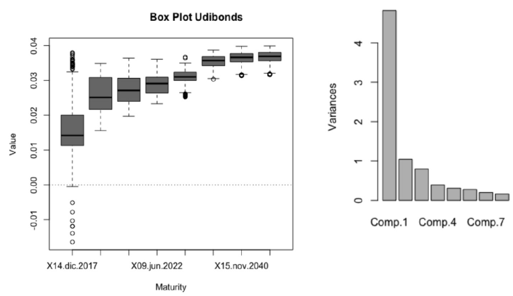
Source: own computations with Banco de Mexico Data.
Figure 3 Inflation-Linked Bonds (Udibonos) Box-Plot and Principal Components
Figure 4 shows the range of the fixed interest rates of the TIIE 28-day swaps during the period and their principal components.
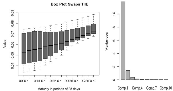
Source: own computations with Bloomberg Data.
Figure 4 TIIE interest-rate swap Box-Plot and Principal Components

Table 1 Swap Interest rates Correlation Matrix
| 3 x 1 | 6 x 1 | 9 x 1 | 13 x 1 | 26 x 1 | 39 x 1 | 52 x 1 | 65 x 1 | 91 x 1 | 130 x 1 | 156 x 1 | 195 x 1 | 260 x 1 | 390 x 1 | |
|---|---|---|---|---|---|---|---|---|---|---|---|---|---|---|
| 3 x 1 | 100% | 87% | 80% | 74% | 65% | 59% | 57% | 55% | 51% | 49% | 48% | 46% | 45% | 44% |
| 6 x 1 | 87% | 100% | 95% | 91% | 85% | 80% | 77% | 75% | 71% | 69% | 67% | 65% | 64% | 64% |
| 9 x 1 | 80% | 95% | 100% | 96% | 92% | 88% | 85% | 84% | 79% | 75% | 73% | 71% | 70% | 70% |
| 13 x 1 | 74% | 91% | 96% | 100% | 95% | 92% | 89% | 88% | 84% | 80% | 79% | 77% | 76% | 76% |
| 26 x 1 | 65% | 85% | 92% | 95% | 100% | 97% | 94% | 94% | 91% | 87% | 86% | 83% | 82% | 82% |
| 39 x 1 | 59% | 80% | 88% | 92% | 97% | 100% | 96% | 95% | 93% | 89% | 88% | 86% | 85% | 84% |
| 52 x 1 | 57% | 77% | 85% | 89% | 94% | 96% | 100% | 96% | 94% | 91% | 90% | 88% | 86% | 86% |
| 65 x 1 | 55% | 75% | 84% | 88% | 94% | 95% | 96% | 100% | 97% | 95% | 94% | 92% | 91% | 91% |
| 91 x 1 | 51% | 71% | 79% | 84% | 91% | 93% | 94% | 97% | 100% | 97% | 96% | 94% | 93% | 93% |
| 130 x 1 | 49% | 69% | 75% | 80% | 87% | 89% | 91% | 95% | 97% | 100% | 99% | 98% | 97% | 97% |
| 156 x 1 | 48% | 67% | 73% | 79% | 86% | 88% | 90% | 94% | 96% | 99% | 100% | 98% | 97% | 97% |
| 195 x 1 | 46% | 65% | 71% | 77% | 83% | 86% | 88% | 92% | 94% | 98% | 98% | 100% | 98% | 98% |
| 260 x 1 | 45% | 64% | 70% | 76% | 82% | 85% | 86% | 91% | 93% | 97% | 97% | 98% | 100% | 100% |
| 390 x 1 | 44% | 64% | 70% | 76% | 82% | 84% | 86% | 91% | 93% | 97% | 97% | 98% | 100% | 100% |
Source: own computations with Bloomberg data.
For the previous computation the simple returns were used in order to apply principal components analysis and obtain the spectral decomposition of the matrix of variance and covariance (Σ).
Where G is an orthogonal matrix composed of the eigenvectors and is the transposed matrix G’ that is also the inverse matrix of G as it is orthogonal, and is a diagonal matrix where each diagonal entry is a non-negative and ordered eigenvalue from highest to lowest, if is a non-negative definite matrix.
Thus the principal components transformation is:
For i = 1,...,n and x i represent the returns of each security cantered to its mean and y i are the new variables that are not correlated.
The analysis of principal components in this document was carried out using the matrix of correlations for each asset class, but it can also be done using the variance-covariance matrix. It is possible to know how many components are enough as they are estimated using the correlation matrix and are at least those with an Eigen-value greater than one. If the analysis is performed using the variance-covariance matrix, it will be necessary to use the Bartlett test for sphericity.
The results obtained using the principal components analysis suggest, as mentioned in several studies, that only the first three components are enough to explain more than 80% of the variance for the different yield curves. In the case of the zero-coupon bond curve, the first three components only explain 77%. This could be explained by different factors. One of them is that the movements in the rates of these instruments are strongly affected by monetary policy and its expectations that directly affect the short end of the curve, in the case of Mexico the Cetes curve. The effects of monetary policy action on long-term interest rates are looser and variable. These behaviors are documented in several papers, such as Roley (1995). In addition, these instruments are less liquid than the instruments in the other curves. The volumes published by Banco de Mexico for these instruments are less than for other instruments and the rotation is low. The low volumes of operations in these instruments can be explained as these instruments are bought and held by mutual funds, pension funds, and some foreign asset managers, according to the statistics published by Banco de México and the U.S. Securities and Exchange Commission.
Table 3 First three principal components analysis for Mexican curves (Standard Deviation)
| Standard Deviation | First Component | Second Component | Third Component |
|---|---|---|---|
| Zero-Coupon Bond | 1.83 | 1.09 | 0.90 |
| Bonds | 3.61 | 1.19 | 0.72 |
| Inflation-linked Bonds | 2.19 | 1.02 | 0.89 |
| Interest-rate swaps | 3.44 | 1.17 | 0.60 |
From the previous results (Figure 6), in which the eigenvectors were obtained for the principal components analysis for the four different curves, it is possible to observe the behavior expected in Litterman (1991).
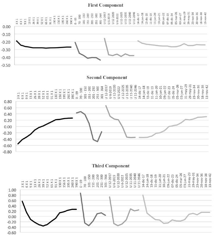
Source: own computations with Bloomberg data.
Figure 6 figure First, Second and Third loadings for each Mexican fixed-income market
The first component can be interpreted as a parallel shift component. The factor loadings are roughly constant among maturities for the bonds and TIIE interest-rate swaps curve, meaning the change in the rate for a maturity is roughly the same for other maturities. In the case of the zero-coupon bonds this behavior is less clear, but for the inflation linked bonds the behavior remains if the first node is excluded. It is worth mentioning that the inflation-linked bonds with less than one year of maturity tend to present disruptions of valuations according to the short-term inflation expectations. Consequently, the first factor accounts for the average rate.
The second component corresponds to the slope of the curve. The factor loadings of the second component have a monotonic change with maturities: changes in long-maturity and short maturity have opposite signs. The second factor consequently accounts for the “slope” across maturities. Even this behavior is consistent in all the markets: the monotonic behavior is increasing for interest rates and bonds and decreasing for the Cetes and inflation-linked bonds.
The third component is the curvature. The factor loadings of the third component are different for the mid-term rates and the average of long- and short-term rates, revealing a curvature resembling the convex shape of the relationship between the rates and their maturities.
Another important property of the use of principal components is that the sum of the variances of the transformed variables is the sum of the eigenvalues. This property will be used for the construction of the indicator of volatility for the different yield curves in the following sections.
Orthogonal GARCH and Volatility Indicator for the Mexican yield curves
Once the principal components are obtained, the problem is reduced to computing a diagonal variance-covariance matrix of dimension 3x3 and then it is possible to compute the variance of the yield curve with the matrix trace. In order to estimate the variance of each component, a GARCH(1,1) was adjusted.
Once more than 80% of the variability for all the markets can be explained, it is possible to use the first three components for each curve, which are linearly independent and therefore not correlated, so as to find a method to estimate the variance of each curve. One possibility is the use of an orthogonal GARCH model, which is a generalization of the GARCH factors introduced by Engle and Rothschild in 1990. This model provides a parsimonious alternative for the estimation of the variance of the curve and for the estimation of variance and covariance of matrices using three univariate GARCH models for their calculation.
The use of the GARCH multivariate using the first three components reduces the problem of estimating variance and covariance in estimating three univariate GARCH models. It must be borne in mind that being linearly independent only guarantees that it is non-conditional non-correlated. Although this assumption is strong, it is necessary to obtain the variance-covariance matrix using the estimates of the GARCH for the diagonal.
Three univariate GARCH models that comprise the diagonal matrix of variances were estimated by this method. For this estimation a GARCH (1,1) with normal distribution is used. The GARCH (1,1) was selected because it is a model commonly used in the literature and because of existing empirical evidence that GARCH models with higher parameters do not substantially improve the precision of estimates, so it was deemed preferable to work with a simpler model:
Where the parameter is the reaction of the market and the parameter is the persistence of the volatility. The sum of both parameters must be less than one to ensure the convergence of volatility forecasts. The orthogonal GARCH is useful to estimate the volatilities of curve nodes with low liquidity or with few data.
For each of the components the stationarity was tested through the assumptions, with 99% Dickey-Fuller test confidence.
For the analysis of the Zero-Coupon Bond Curve, a GARCH(1,1) was adjusted for each of the first three principal components. The estimation was significant for each parameter and for the three GARCH models. The Dickey-Fuller test was also performed in order to test stationarity.
Table 5 Zero-coupon bonds GARCH estimation
| 1º Component | 2º Component | 3º Component | ||||
|---|---|---|---|---|---|---|
| Coefficient | t-statistic | Coefficient | t-statistic | Coefficient | t-statistic | |
| ϖ | 5.56e-01 | 3.357 | 3.67e-01 | 3.653 | 7.30e-02 | 3.172 |
| α | 3.86e-01 | 5.139 | 2.93e-01 | 4.246 | 3.28e-01 | 5.141 |
| β | 5.26e-01 | 6.771 | 3.81e-01 | 3.034 | 6.29e-01 | 11.176 |
| Dickey-Fuller | p-value | 10-3 | p-value | 10-3 | p-value | 10-3 |
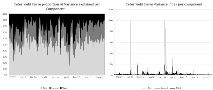
Figure 7 Cetes yield curve Variance estimated using the orthogonal GARCH for the principal components
It is observed that the first and second components have the highest volatility and react to the changes in monetary policy and that in November 2016 the variance of each component reached its maximum after the United States Presidential Elections. The first component that represents the parallel shift accounts for more than 60% of the variance. In addition, it is observed that in general there is no high volatility in this market.
In addition, the same analysis was performed for the Nominal Bonds, Inflation-linked, and TIIE interest-rate swaps Curves, for which a GARCH(1,1) was adjusted for each one of their first three principal components. The estimation was significant for each parameter and for the three GARCH. In addition, the Dickey-Fuller test was performed in order to test stationarity.
Table 6 Nominal bonds GARCH estimation
| 1° Component | 2° Component | 3° Component | ||||
|---|---|---|---|---|---|---|
| Coefficient | t-statistic | Coefficient | t-statistic | Coefficient | t-statistic | |
| 1.1788 | 2.925 | 3.60e-01 | 1.455 | 2.174e-01 | 3.635 | |
| 1.956e-01 | 4.568 | 5.27e-01 | 4.447 | 3.96e-01 | 3.924 | |
| 7.197e-01 | 14.048 | 3.31e-01 | 1.388 | 2.394e-01 | 2.002 | |
| Dickey-Fuller | p-value | 10-3 | p-value | 10-3 | p-value | 10-3 |
Source: own computation with Banco de México data amd Bloomberg data.
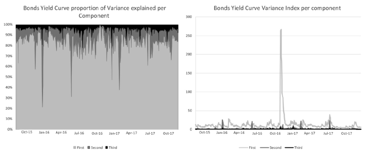
Figure 8 Nominal Bond yield curve Variance estimated using the orthogonal GARCH for the principal components.
For the GARCH models estimated for the nominal bond curve, all the parameters are significant and the first component explains approximately 90% of the variance, with the exception of particular periods in which the biggest change was observed in the slope of the curve. These movements relate to changes in the monetary policy, because the Central Bank of Mexico had a tight cycle from December 2015 to December 2017. It is also worth mentioning that the effect of the presidential election in the bond curve was absorbed by the parallel shift.
Table 7 Inflation-linked bonds GARCH estimation
| 1° Component | 2° Component | 3° Component | ||||
|---|---|---|---|---|---|---|
| Coefficient | t-statistic | Coefficient | t-statistic | Coefficient | t-statistic | |
| ϖ | 2.42e-01 | 1.379 | 2.08e-02 | 1.603 | 7.79e-03 | 1.293 |
| α | 1.69e-01 | 3.774 | 1.73e-01 | 4.972 | 2.71e-01 | 6.040 |
| β | 7.95e-01 | 12.207 | 8.34e-01 | 25.029 | 7.94e-01 | 27.994 |
| Dickey-Fuller | p-value | 10-3 | p-value | 10-3 | p-value | 10-3 |
Source: own computation with Banco de México data
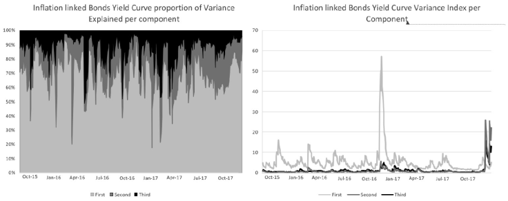
Figure 9 Inflation-linked Bond yield curve Variance estimated using the orthogonal GARCH for the principal components
As in the other markets, the biggest component for the variance was the parallel shift that also reached its maximum after the US presidential elections in November 2016. The parameters obtained are also significant for each model. It is also relevant that there is an increase in the second and third component at the end of 2017. This increment was observed as the inflation and the inflation expectations increased. Furthermore, there is an effect of valuation in the first node of the inflation-linked curve as the rate tends to increase or decrease adapting to the inflation expectations.
Table 8 TIIE interest-rate swaps curve GARCH estimation
| 1º Component | 2º Component | 3º Component | ||||
|---|---|---|---|---|---|---|
| Coefficient | t-statistic | Coefficient | t-statistic | Coefficient | t-statistic | |
| ϖ | 1.234 | 2.386 | 1.057 | 8.982 | 4.13e-02 | 3.128 |
| α | 3.14e-01 | 4.593 | 3.24e-01 | 5.176 | 4.88e-01 | 5.816 |
| β | 6.20e-01 | 7.168 | 0 | -- | 5.728e-01 | 10.326 |
| Dickey-Fuller | p-value | 10-3 | p-value | 10-3 | p-value | 10-3 |
Finally, for the TIIE interest-rate swaps curve the parameters are significant with the exception of the for the second component. The behavior of the interest-rate swap curve is very similar to the behavior observed in the nominal-bond curve. For both, the first component, the parallel shift, represents more than 80% of the variability and reached its maximum in November 2016 after the presidential elections in the USA. Also, it is observed that the second component reacts to the monetary policy decision as it was observed that the Mexican interest-rate curve reacted to the increments in the one-day reference rate of Banco de Mexico by showing a flatter movement. In addition, the investors used the first nodes of the curve to hedge their position against further increments in the monetary policy reference rate.
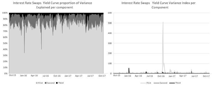
Source: own computation with Banco de México data.
Figure 10 TIIE swap interest-rate curve variance estimated using the orthogonal GARCH for the principal components
With the variances for each of the components an index is built for the volatility of each asset class, which is the square root of the sum of the variances of each of the annualized basis components. It is worth mentioning that the main source of variability comes from the first component, as expected. This also highlights how in times of stress the second component can be increased significantly. The index is computed basically using the square root of the trace of the variance-covariance matrix:

Variance and Covariance Matrix
The advantage of using the orthogonal GARCH model is that it generates the simple form of variance and covariance matrices for different terms without assuming that the volatilities and correlations remain constant. This method ensures that the obtained matrices are semi-defined positive, which is useful when using the variance-covariance matrices for portfolio optimization or for the calculation of the value at risk.
According to Engle (2000), orthogonal GARCH performs quite well based on diagnoses made by evaluating precision in forecasts of the correlations. This is relevant as the GARCH models react rapidly to changes in the market condition whose lag could be significant in the case of historical computation and also this method smoothes the changes in the market conditions. However, without using this approach based on principal components analysis and orthogonal GARCH, a high dimension multivariate GARCH will be required to adjust the market condition for each variance and covariance. Thus, among the advantages of the estimation of these matrices is that the covariance between the nodes of the curve increases in periods of volatility in the markets, as estimated by the three GARCH variance increases, which are also increases in the correlation between the nodes. Finally, it is common that in the market some instruments present a misevaluation or liquidity problems that may affect the computation of the variance-covariance matrix. However, using the methodology proposed, the matrix obtained reflects only the three most important factors for investors.
To estimate the variance-covariance matrix (), the first three eigenvectors obtained by the principal components analysis (P) are multiplied by the diagonal matrix of variances estimated with GARCH (S).
Table 9 Example of the variance-covariance matrix estimated for the TIIE interest-rate curve
| 3 X 1 | 6 X 1 | 9 X 1 | 13 X 1 | 26 X 1 | 39 X 1 | 52 X 1 | 65 X 1 | 91 X 1 | 130 X 1 | 156 X 1 | 195 X 1 | 260 X 1 | 390 X 1 | |
| 3 X 1 | 0.625 | 0.567 | 0.516 | 0.458 | 0.377 | 0.323 | 0.294 | 0.268 | 0.235 | 0.209 | 0.199 | 0.185 | 0.178 | 0.174 |
| 6 X 1 | 0.567 | 0.575 | 0.558 | 0.525 | 0.474 | 0.435 | 0.411 | 0.389 | 0.357 | 0.327 | 0.317 | 0.300 | 0.293 | 0.290 |
| 9 X 1 | 0.516 | 0.558 | 0.560 | 0.541 | 0.506 | 0.476 | 0.454 | 0.433 | 0.402 | 0.370 | 0.359 | 0.341 | 0.333 | 0.330 |
| 13 X 1 | 0.458 | 0.525 | 0.541 | 0.535 | 0.516 | 0.495 | 0.479 | 0.463 | 0.436 | 0.408 | 0.398 | 0.381 | 0.374 | 0.372 |
| 26 X 1 | 0.377 | 0.474 | 0.506 | 0.516 | 0.519 | 0.512 | 0.502 | 0.495 | 0.476 | 0.455 | 0.446 | 0.433 | 0.427 | 0.425 |
| 39 X 1 | 0.323 | 0.435 | 0.476 | 0.495 | 0.512 | 0.512 | 0.506 | 0.504 | 0.490 | 0.473 | 0.466 | 0.454 | 0.449 | 0.448 |
| 52 X 1 | 0.294 | 0.411 | 0.454 | 0.479 | 0.502 | 0.506 | 0.504 | 0.507 | 0.497 | 0.486 | 0.481 | 0.470 | 0.466 | 0.465 |
| 65 X 1 | 0.268 | 0.389 | 0.433 | 0.463 | 0.495 | 0.504 | 0.507 | 0.518 | 0.515 | 0.513 | 0.509 | 0.501 | 0.498 | 0.498 |
| 91 X 1 | 0.235 | 0.357 | 0.402 | 0.436 | 0.476 | 0.490 | 0.497 | 0.515 | 0.518 | 0.524 | 0.522 | 0.517 | 0.516 | 0.516 |
| 130 X 1 | 0.209 | 0.327 | 0.370 | 0.408 | 0.455 | 0.473 | 0.486 | 0.513 | 0.524 | 0.542 | 0.542 | 0.541 | 0.542 | 0.542 |
| 156 X 1 | 0.199 | 0.317 | 0.359 | 0.398 | 0.446 | 0.466 | 0.481 | 0.509 | 0.522 | 0.542 | 0.543 | 0.543 | 0.544 | 0.544 |
| 195 X 1 | 0.185 | 0.300 | 0.341 | 0.381 | 0.433 | 0.454 | 0.470 | 0.501 | 0.517 | 0.541 | 0.543 | 0.544 | 0.546 | 0.547 |
| 260 X 1 | 0.178 | 0.293 | 0.333 | 0.374 | 0.427 | 0.449 | 0.466 | 0.498 | 0.516 | 0.542 | 0.544 | 0.546 | 0.549 | 0.549 |
| 390 X 1 | 0.174 | 0.290 | 0.330 | 0.372 | 0.425 | 0.448 | 0.465 | 0.498 | 0.516 | 0.542 | 0.544 | 0.547 | 0.549 | 0.549 |
Conclusions
The use of the orthogonal GARCH model and its accuracy has been validated empirically to model assets that have a high correlation, as is the case for the Mexican fixed -income securities, financial futures curves such as oil or gasoline futures, or even emerging markets fixed-income curves. The empirical evidence suggests that the methodology proposed has virtually the same performance with multivariate GARCH models and, by requiring a smaller number of parameters to estimate, takes less time and prevents some problems when producing the estimations as there is a parsimonious number of parameters. However, there are some relevant points to consider. Alexandre (2001) mentions that it is necessary to take special care when assets are not highly correlated. Additionally, she mentions that special care must be taken in the first calibration, and then once the calibration is successful it can be used on a daily basis without the need to recalibrate.
The index constructed from the variances of the first three principal components allows policy makers to have an indicator that shows the volatility of the different fixed-income markets and how these markets react to new information and reflect the market conditions without the need to monitor the volatility of each node. Additionally, each of the three components provides valuable information to identify whether the increase in volatility is due to a change in the parallel-curve shift or its slope, as can occur after monetary policy decisions, or if it comes from changes in the curvature.
Finally, as an extension of the paper the GARCH will be worked with residuals with a different distribution, which is an interesting extension because in a world with linked instruments and markets, another characteristic like asymmetry can be expected. Another extension is the application of this study for an index of emerging markets.

