


Servicios Personalizados
Revista
Articulo
 texto en
  Inglés (pdf)
 Artículo en XML
 Referencias del artículo
 Enviar artículo por email
Indicadores
-
 Citado por SciELO
 -
 Accesos
Links relacionados
-
 Similares en
SciELO
Similares en
SciELO
Compartir

 Permalink
Contaduría y administración
versión impresa ISSN 0186-1042
Contad. Adm vol.64 no.2 Ciudad de México abr./jun. 2019 Epub 10-Dic-2019
https://doi.org/10.22201/fca.24488410e.2018.1848
Determinants of capital structure: an empirical study of the manufacturing sector at Ecuador
1 Universidad Autónoma de Madrid, España.
2 Universidad de Especialidades Espíritu Santo, Ecuador
The objective of this study is to discover the determinants of the capital structure of 304 companies in the manufacturing sector of Guayaquil, during the period 2012-2016 and which theory best condenses the financing decisions of companies. The importance of it lies in verifying the determinants of indebtedness in companies in a developing country and comparing the results with the predictions of the Trade-off and the Pecking Order theories. As a methodology, a panel data structure has been used together with a fixed effects model. After reviewing the literature, an Ordinary Least Squares regression model was used to discover the correlation and statistical significance between the dependent variable (debt ratio) and a set of selected independent variables. In this study, the Pecking Order theory had a greater explanatory power than the Trade-off theory. However, no statistical evidence was found to support the importance of growth expectations on the corporate capital structure.
JEL Codes: G32; C12
Keywords: Financing; capital structure; manufacturing; leverage; Trade-off; Pecking Order
El objetivo de este estudio es descubrir los determinantes de la estructura de capital de 304 empresas del sector manufacturero de Guayaquil, durante el periodo 2012-2016 y qué teoría condensa mejor las decisiones de financiación de las empresas. La importancia del mismo, reside en verificar los determinantes del endeudamiento en empresas de un país en vías de desarrollo y comparar los resultados con las predicciones de las teorías sobre el Equilibrio Estático y sobre la Jerarquía Financiera. Como metodología se ha empleado una estructura de datos de panel junto a un modelo de efectos fijos. Tras la revisión de la literatura se ha utilizado un modelo de regresión de Mínimos Cuadrados Ordinarios para descubrir la correlación y significación estadística entre la variable dependiente (ratio de endeudamiento) y un con-junto de variables independientes seleccionadas. En este estudio, la teoría de la Jerarquía Financiera tuvo mayor poder explicativo que la del Equilibrio Estático. Sin embargo, no se encontró evidencia estadística que sustente la importancia de las expectativas de crecimiento sobre la estructura de capital corporativa.
Códigos JEL: G32; C12
Palabras clave: Financiamiento; estructura de capital; manufactura; endeudamiento; Equilibrio Estático; Jerarquía Financiera
Introduction
In recent years, it has been observed that one of the main objectives of managers is to increase the value of the company for shareholders. Naturally, a company requires assets, whether tangible or intangible, to carry out its business, create value, and achieve its business objectives. The financing of these assets can be done through three options: a) obtaining debt (bank or corporate); b) shareholder contribution; and c) own funds. Deciding on the mix or combination of debt and capital can be a difficult exercise because high indebtedness could increase the probability of bankruptcy, simultaneously reducing the payment of taxes and, therefore, providing a tax advantage. On the other hand, little debt would imply a reduction in yield due to increased tax pressure and issues leading to over-investment problems, followed by a reduction in the returns of shareholders.
The importance of studying the capital structure of companies lies in the generation of models that can summarize and predict the most relevant factors that influence the decision to obtain an “optimal” capital structure that allows the efficient use of resources. It was Modigliani and Miller who in 1958 developed the first theory about capital structure, where they indicated that in a perfect market the value of the firm has no relation to its capital structure, and that taxes, cost of capital, information asymmetry, and bankruptcy costs would not affect either, but that its value is given by the value of the assets it possessed (Modigliani & Miller, 1958).
However, the problem with the theories of Modigliani & Miller is that they assume unrealistic scenarios. In a recent work by (Serrasqueiro, Matias, & Salsa, 2016), they indicate that the tax advantages generated by the use of debt added substantial value to companies, mainly by saving on tax payments. Furthermore, Miller (1977) included in his work the effect of taxes in the analysis and determined that taxes only affect at a macro level and not individual companies. DeAngelo & Masulis (1980) indicated that not only could the payment of taxes be reduced through indebtedness, but that there were substitutes (depreciation, amortization, tax credits for investment, among others) that did not increase the liabilities of corporations. On the other hand, Myers (1974) argued that corporations would prefer debt over equity for two reasons: 1) the cost is lower, and 2) investors would consider the company to be overvalued and could restrict the issuance of new capital.
From the above emerged a great number of alternative theories and models, such as including market imperfections and allowing corporate directors to make financial decisions on an objective and proven basis. Several of these have largely failed, since economic and financial conditions may be very different depending on the region studied, leading to a neutralization of the validity of such models (Booth, Aivazian, Demirguc-Kunt, & Maksimovic, 2001). In addition, the theories differ in their emphasis and no consensus has been reached among academics (Sheikh & Wang, 2011) regarding which best synthesizes the financial behavior of the companies. An example is that research with alternative approaches has studied the relationship between the compensation of the directors and the capital structure of the companies they run. It was found that the market value of capital and debt decreases when the director is changed, as well as the expected cash flow is higher in companies that do not change their directors. On the contrary, maintaining the director would have a positive correlation with company size, leverage, salary compensation, and cash flow (Berkovitch, Israel, & Spiegel, 2000).
There are two main theories that seek to address the issue of capital structure from different perspectives and different predictions. The first is the Trade-off Theory of Capital Structure, which emphasizes taxes, financial difficulties, and conflict of interest; and the second is the Pecking Order Theory, which emphasizes information asymmetry among directors, shareholders and creditors, and financial independence as determinants of capital structure.
The objective of this research is to discover the determinants of the capital structure of 304 companies in the manufacturing sector of Guayaquil during the period of 2012-2016 and to identify which theory best summarizes the financing decisions of the companies. The importance of this lies in verifying the determinants of indebtedness in companies in a developing country and comparing the results with the predictions of the theories on Capital Structure and on the Pecking Order. In other words, to check the predictions of these two theories in order to generate evidence to determine their explanatory power in companies in developing Latin American countries. In this sense, it is also expected that the results of this work will contribute to the general knowledge about the financial conduct of companies in developing countries and, through the results obtained, to the theories of capital structure.
Theoretical Framework
Capital Structure: theories
The work of Modigliani & Miller was the first to expose what exists behind the decisions of the capital structure of corporations. In their work, they argued that in a perfect market the value of companies is not influenced by the decisions of the capital structure. This implied that the existence of taxes, agency costs, capital costs, bankruptcy costs, and information asymmetry had no relevance in the debt-equity mix and that their value depended on their assets instead.
However, there were certain problems in their theory: it did not integrate real-life situations, i.e. it did not include market imperfections. Years later, both authors published an article indicating that they had made a mistake by not adapting their theories to real conditions (Modigliani & Miller, 1963). Both recognized the particular tax advantages of using debt, since incurring debt generates interest that is deductible from the payment of taxes. In other words, they asserted that taxes were determinants of capital structure, contrary to their previous research work. However, they warned that, despite the advantages of indebtedness, companies should not incur the maximum amount of debt potentially guaranteed by their assets, since this could increase the likelihood of bankruptcy.
Initially, two theories were mentioned in this paper: The Trade-Off Theory of Capital Structure (TOT) and the Pecking Order Theory (POT). Each theory presents different predictions, i.e. different effects of the determinants in the debt-equity mix.
There are studies that have indicated that the expected cost of bankruptcy does influence the capital structure (Warner, 1977). Werner (1977), after analyzing the capital structure of railway companies, concluding that bankruptcy costs have an inverse relationship with the market value of the company, that is, costs fall when the value of the company increases, and could become 1% of the value of the company. Modigliani & Miller (1963) recognized the particular tax advantages of using debt, since incurring debt generates interest that is deductible from the payment of taxes. In other words, they discovered that taxes were determinants of capital structure. However, they warned that, despite the advantages of indebtedness, companies should not incur the maximum amount of debt potentially guaranteed by their assets, since this would mainly increase the probability of bankruptcy.
According to the Trade-Off Theory of Capital Structure (TOT), the capital structure of companies is determined by the cost-benefit evaluation with respect to the use of debt to finance operations (Serrasqueiro & Caetano, 2015). According to the TOT, financing decisions depend on three aspects: a) taxes, b) bankruptcy costs, and c) agency costs (Acaravci, 2016). This theory mentions that companies balance the tax advantages obtained by debt against the probabilities of bankruptcy (Warner, 1977). In other words, it tries to predict the optimal level of debt that administrators should set in order to minimize bankruptcy costs and maximize tax advantages (Serrasqueiro, Matias, & Salsa, 2016; DeAngelo & Masulis, 1980).
This target and optimal level of debt would be inversely related to the expected costs of bankruptcy and the number of fiscal shields not generated by debt (Bradley, Jarrell, & Kim, 1984). The latter were included in the model by Miller (1977) and by (DeAngelo & Masulis, 1980). Other studies have shown that companies with zero or little debt have higher tax spreads, indicating no need for fiscal shields (Kolay, Schallheim, & Wells, 2013).
On the other hand, this theory indicates that agency problems tend to be reduced through indebtedness, since indebtedness would serve as a disciplinary mechanism for managers because the debt burden would prevent the inefficient use of cash (Fama & French, 2002). The reason indebtedness functions as a control mechanism for directors is that debt repayment requires constant and periodic outflows of cash in the form of capital and interest, thereby limiting the cash available only for strictly necessary disbursements. Cash constraints, in certain contexts, could prevent the director from deviating from the objectives of shareholders and their commitment to them. Managers and directors are generally motivated to achieve their own objectives, which could stray from the maximization of the value of the company for shareholders (Eriotis, Vasiliou, & Ventoura-Neokosmidi, 2007). Financial leverage would reduce conflicts between shareholders and the director, but increase conflicts between shareholders and creditors (Frank & Goyal, 2009; Myers, 1977) given that the right to cash flow of the company would be conditioned by the debt-equity combination in force at the time.
Regarding the Pecking Order Theory (POT), it argues that companies should not pursue an optimal level of debt (Myers, 1984; Myers & Majluf, 1984). In other words, it attaches little importance to external financing and rather prioritizes financing from its own resources. Furthermore, it points out that financing decisions follow a pecking order that is governed by the implicit cost of access to and availability of capital (Myers, 1984). Consequently, companies would prefer to use retained equity, followed by capital injections from existing or new partners, and finally debt.
The use of debt would be conditioned by the existence of equity, that is to say, the debt would be used when the equity is exhausted. This theory focuses on the relationship between information asymmetry and financing options. Directors are the ones who have access to “inside” information regarding the future of the company (Chen & Chen, 2011), so that it is they who have a clearer view of the risks the company would incur under any of the scenarios, and what the effects would be on shareholder performance. This obviously influences financial decisions, mainly because shareholders expect the value of the company to be maximized. Of course, under this hypothesis the risk of the project or projects in which the funds are placed is not being considered, but from the point of view of maximizing the value of the company, financing through equity is the best option. On the other hand, if investors believe that the company is undervalued, they will be reluctant to allow the director to issue new capital, so they will choose the use of debt (Ferrer & Tanaka, 2009) to prevent the dilution of participation.
Information asymmetry is evident between directors and creditors when the credit terms between creditor and debtor depend on the market value of the collateral. If the company has a high value collateral, the creditor will be more willing to request less information about the condition of the company because the value of the collateral is “sufficient” (Leland, 1998), and assumes that the risk of bankruptcy is lower, something that would benefit both the creditor and the debtor. Thus, under this scenario, the cost of capital is reduced. However, at the same time, there would be conflicts between shareholders and creditors due to the transfer of wealth from the shareholder to the creditor (Jorgensen & Terra, 2003).
Empirical evidence in Latin America
Padilla Ospina, Rivera Godoy, & Ospina Holguín (2015) conducted a study of SMEs in Colombia, in the period of 2007-2011, in which they analyzed 309 companies seeking to determine the relationship and incidence of six independent variables (age of the company, tangibility, business risk, profitability, roe, and size) on corporate indebtedness, whether short or long-term. They used panel data analysis, accompanied by the fixed-effect model. They found a positive and significant relationship between debt and tangibility, as well as with profitability and company size.
Hernández & Ríos (2012) analyzed the determinants of the capital structure of 14 Mexican companies belonging to the food industry. The study period was 2000 to 2009. The following independent variables were analyzed: company size, profitability, business risk and tangibility. The dependent variable was the level of indebtedness measured as total debt/total equity. Their findings were “that tangible assets are the main variable that these companies consider to define their financing decisions”.
Tenjo, López, & Zamudio (2006) conducted a study in Colombia, where they sought to estimate the incidence of five independent variables (profitability, sales [used as a size proxy], asset tangibility, sector, and idiosyncratic characteristic) on the ratio of total indebtedness, measured as total debt over total assets. An important aspect of the study was that they isolated it within a context of crisis that existed in the country in recent years. The study period covered the years 1996 to 2002 and involved approximately 7,326 companies per year. They used a method called Quantile Regression that “uses the full distribution of the indebtedness of the companies, conditional on a set of explanatory variables”. In general terms, they found a negative relationship between the level of debt and profitability; a positive relationship between the size of the company and the level of debt; and a negative relationship between the tangibility and the level of debt. The results were consistent with the predictions of the Pecking Order Theory.
Paredes, Ángeles, & Flores (2016) studied 14 publicly traded mining companies across five Latin countries: Mexico, Chile, Colombia, Peru, and Brazil. The study period was 2004. They considered five variables: total debt ratio (dependent variable), tangibility of assets, company size (natural logarithm of sales), growth opportunities, and profitability. They used a panel data structure alongside the fixed-effects model. Tangibility, size, and profitability were found to negatively and significantly influence the level of debt of mining companies. Such results were more consistent with the Pecking Order Theory.
Franco, López, & Muñoz (2010) sought to establish “the determinants of the indebtedness of national manufacturing companies [...]” in Uruguayan companies. They chose to use multiple linear regression as a tool to work with cross-sectional data over a period of three years: 2004, 2005, and 2006. The sample size was 38 for the first two years and 30 for the last year. They took into account 9 independent variables and 1 dependent variable. The independent variables were: size, tangibility, profitability, tax benefit, export orientation, equity, cash flow, impact of the sector, and age of the company. The dependent variable was the total debt ratio. Only the variable “cash flow” had a significant and negative relationship with indebtedness.
Data and Methodology
To achieve the established objectives, an exploratory, empirical, and quantitative study was proposed on small and medium manufacturing enterprises in Guayaquil, during the period of 2012-2016. The population under study has been obtained from the companies associated with the Chamber of Small Industry of Guayas (CAPIG for its acronym in Spanish)1. In order to carry out the study, the 304 companies for which sufficient information was available from the five years under study were taken.
CAPIG groups its partners in 25 different sectors. Within the final sample, there are only 5 sectors that group more than 50% of the companies: Chemical (18.42%), Food and Beverages (10.20%), Metalworking (8.88%), Services (7.57%), and Plastics and Rubber (6.91%). In 2016, the sales of the sampled companies reached $1.38 billion dollars (1.43% of GDP) as a whole, while the nominal Ecuadorian GDP of the same year, according to data from the World Bank, was $97.8 billion dollars.
This study has considered only companies incorporated according to the regulations of the Superintendence of Companies and Securities, eliminating individual companies as there is no public information on their financial situation. Generally, similar research has focused on analyzing listed companies. However, the Ecuadorian stock market is not representative in comparison to other economies, so the study has focused on SMEs to be more useful, from a comparative point of view, with that of other surrounding countries.
Since the time interval runs from 2012 to 2016, the first step was to eliminate companies with incomplete information and fewer years of financial information than the study required. The financial statements and balance sheets of the available companies were then collected, from which all the data necessary for the study were extracted. All data were obtained through the web page of the Superintendence of Companies, Securities and Insurance of Ecuador2 and worked with securities at year-end. Microsoft Excel was used to sort and adapt the data in the form of panel data, for later export to the Stata v. 143 statistical tool, with which the statistical models for the study were generated together with the corresponding statistical tests.
Determinant variables of the capital structure
The variables analyzed and which determine indebtedness for the companies in the sample are the following:
Profitability: The Trade-Off Theory of Capital Structure predicts a positive relationship between the indebtedness and profitability of the company. The assumption of this theory is that the company, being highly profitable, can incur more debt, which translates into a growing payment of interest that are deducted from taxes (Kouki & Said, 2012; Padilla Ospina, Rivera Godoy, & Ospina Holguin, 2015).
On the other hand, the Pecking Order Theory predicts a negative relationship between indebtedness and profitability. It assumes that companies prefer to use their own resources rather than borrow them; therefore, the more profitable the company, the less debt will be used as a financial resource. Many studies have demonstrated through empirical experiments the validity of the POT (Serrasqueiro, Matias, & Salsa, 2016; Saeedi & Mahmoodi, 2009; Acaravci, 2016; Serrasqueiro & Caetano, 2015; Booth, Aivazian, Demirguc-Kunt, & Maksimovic, 2001; Tenjo, López, & Zamudio, 2006; Paredes, Ángeles, & Flores, 2016). This will be measured with the following formula:
Size: The Trade-Off Theory of Capital Structure predicts a positive relationship between size and indebtedness. This relationship would exist on the assumption that a large company is much more diversified than a smaller one. Diversification, per se, would reduce 1) the risk of bankruptcy, and 2) income volatility. On the other hand, with large companies there is a greater bargaining power with creditors. Several studies have demonstrated this positive relationship (Acedo, Alútiz, & Ruiz, 2012; Kouki & Said, 2012; Eriotis, Vasiliou, & Ventoura-Neokosmidi, 2007; Serrasqueiro & Caetano, 2015; Padilla Ospina, Rivera Godoy, & Ospina Holguin, 2015; Tenjo, López, & Zamudio, 2006), while others have shown that there is no statistically significant relationship (Tanaka, 2008; Hernández & Ríos, 2012).
On the other hand, the POT predicts a negative relationship. The main argument is that large companies have better and easier access to capital markets, leaving aside debt. They are more willing to provide more and better information to potential investors than small companies. Another important fact is that because they are large, they have higher retained earnings to finance themselves (Saeedi & Mahmoodi, 2009; Acaravci, 2016; Sultan & Adam, 2015; Paredes, Ángeles, & Flores, 2016). This will be measured with the following formula:
Tax shields not generated by debt (TSNGD4): The TOT predicts a negative relationship between indebtedness and TSNGD. Despite the fiscal advantages offered by the use of debt, DeAngelo & Masulis (1980) suggest that TSNGD can be almost perfect substitutes for debt to reduce tax payments. There is a discrepancy regarding the effect of TSNGD on capital structure: several researches suggest a positive effect (Serrasqueiro, Matias, & Salsa, 2016; Serrasqueiro & Caetano, 2015), as well as negative and in other cases there is no effect whatsoever (Saeedi & Mahmoodi, 2009; Acaravci, 2016; Titman & Wessels, 1988). This will be measured with the following formula:
Tangibility: The TOT predicts a positive effect of the tangibility of assets against the debt ratio, because the high value of assets is more appreciated by creditors and can be used as collateral to incur more debt. The literature suggests two reasons: 1) agency costs between debtor and creditor are reduced when assets have high market value, and 2) a high collateral value reduces the likelihood of bankruptcy, and even if this were to happen, the creditor would incur less risk of not recovering the debt.
Conversely, the POT predicts a negative relationship between tangibility and the level of debt, because it focuses on the use of domestic resources to finance itself, so following this logic, it rules out debt as an option. The results of several studies are mixed: negative effects have been demonstrated (Serrasqueiro, Matias, & Salsa, 2016; Kouki & Said, 2012; Saeedi & Mahmoodi, 2009; Titman & Wessels, 1988; Booth, Aivazian, Demirguc-Kunt, & Maksimovic, 2001) as well as positive ones (Huang & Song, 2006; Hernández & Ríos, 2012; Padilla Ospina, Rivera Godoy, & Ospina Holguin, 2015). This will be measured with the following formula:
Growth opportunities: The TOT predicts a negative relationship between indebtedness and growth opportunities. According to the TOT, companies with expected high growth have fewer tangible assets that can serve as debt collateral, so they prefer-and need-to be financed through their own resources or external capital. Consequently, their level of debt tends to be very low: large investment opportunities aggravate agency problems between shareholders/ directors and creditors, as well as bankruptcy costs (Myers, 1984), hindering debt financing.
Several researches have supported the TOT hypothesis (Serrasqueiro, Matias, & Salsa, 2016; Eriotis, Vasiliou, & Ventoura-Neokosmidi, 2007). Conversely, Mou (2011), Serrasqueiro & Caetano (2015), and Titman & Wessels (1988) found no significant relationship between both variables.
In contrast, the POT predicts a positive relationship between variables. Companies with large growth opportunities require more funds to acquire assets. When equities are depleted, companies prefer debt rather than capital to finance themselves, because large investments usually carry greater risks. Several empirical studies have supported this hypothesis (Saeedi & Mahmoodi, 2009; Kouki & Said, 2012; Acaravci, 2016). This will be measured with the following formula:
Liquidity: The TOT predicts a positive relationship by arguing that companies with high liquidity ratios have a greater capacity to pay obligations on time, so that companies with high liquidity should ask for more debt (Serrasqueiro, Matias, & Salsa, 2016).
However, the POT suggests a negative relationship between liquidity and indebtedness. The logic behind this proposes that companies first use [and prefer] retained earnings rather than issue instruments to raise capital. Previous empirical studies support this assumption (Serrasqueiro, Matias, & Salsa, 2016; Saeedi & Mahmoodi, 2009; Eriotis, Vasiliou, & Ventoura-Neokosmidi, 2007). This will be measured with the following formula:
Both the variables and the methodology of this research have been used and contrasted in previous studies such as those by (Booth, Aivazian, Demirguc-Kunt, & Maksimovic, 2001; Titman & Wessels, 1988; Jorgensen & Terra, 2003; Frank & Goyal, 2009; Rajan & Zingales, 1995; Sheikh & Wang, 2011). This makes it possible to compare with other studies conducted in different countries and industries, as there is a lack of information regarding the determinants of capital structure in underdeveloped and developing countries, mainly in Latin America and parts of Asia.
Therefore, the research-dependent variable is the “total debt (DR) ratio”, measured as total debt / total assets. Said variable would be explained by the following variables:
Table 1 List of independent/explicative variables.
| Variables | Descripción |
| RENT | Rentabilidad = Cost effectiveness |
| TAM | Tamaño = Size |
| EFND | Escudos fiscales no generados por deuda = Tax shields not generated by debt |
| TANG | Tangibilidad = Tangibility |
| LIQ | Liquidez = Liquidity |
| OC | Oportunidades de crecimiento = Growth opportunities. |
Source: own elaboration.
Therefore, in this research, according to the objectives set and based on the variables explaining indebtedness, the following hypotheses are formulated:
List of hypotheses to be contrasted.
| H1: | There is a positive relationship between profitability and indebtedness. |
| H2: | There is a negative relationship between profitability and indebtedness. |
| H3: | There is a positive relationship between size and indebtedness. |
| H4: | There is a negative relationship between size and indebtedness. |
| H5: | There is a positive relationship between the indebtedness and the tax shields not generated by debt. |
| H6: | There is a positive relationship between tangibility and indebtedness. |
| H7: | There is a negative relationship between tangibility and indebtedness. |
| H8: | There is a negative relationship between indebtedness and growth opportunities. |
| H9: | There is a positive relationship between growth opportunities and indebtedness. |
| H10: | There is a negative relationship between liquidity and indebtedness. |
| H11: | There is a positive relationship between liquidity and indebtedness. |
Source: own elaboration.
To contrast these hypotheses, three different models were used: a) Ordinary Least Squares (OLS) Model, b) Fixed Effects Model, and c) Random Effects Model, to estimate the effect of each explanatory variable on the dependent variable, debt ratio, as well as the statistical significance of each of them in each model. An error level of 5% (0.05) was considered, together with a confidence level of 95%. The equation of the three models, the OLS, fixed, and random effects, are presented below in the same order:
Where i is the company, t is the year, ε it is the stochastic error of company i in time t, and μit is the error term of company i in time t.
The main problem of using the OLS method to analyze panel data is that this technique does not take into account the unobservable effects specific to each company; effects that may vary over time. The analysis mechanism involves grouping together all the observations and assuming that each piece of data, regardless of the period to which it belongs, is an observation that does not take into account each individual as such. This could cause bias and inconsistency in estimates. Several studies suggest that OLS should not be used to address this situation with this tool (Serrasqueiro, Matias, & Salsa, 2016; Labra & Torrecillas, 2014; Paredes, Ángeles, & Flores, 2016).
That said, fixed effects and random effects models were run, and then the Hausman test was performed to determine which of the two models fits best.
According to the literature, there is a possibility of correlating unobserved variables with model variables. Thus, deciding which model to use depends on the existence of that correlation: if there is no correlation between the unobserved individual effects of the companies with the independent variables, it is recommended to address the problem using the random effects model. Otherwise, it is recommended to use the fixed effects model. The advantage of using the fixed effects model is that it does consider the individuality of companies over time, allowing the intercept to vary for each company (Sheikh & Wang, 2011).
x 2). This test compares the coefficients of both models to determine whether or not the differences present are significant. The null hypothesis (Ho) of the test indicates that there is no difference between the coefficients of the model, that is, there is no correlation between the x 2>0.05 the null hypothesis is rejected. Consequently, it is decided that the most efficient model is that of random effects. Otherwise, the fixed effects model is chosen (Labra & Torrecillas, 2014).
The presence of multicollinearity between variables was reviewed, i.e. whether there is a perfect linear relationship between one or more of the explanatory variables. The problem with multicollinearity, according to the theory, is that if it is perfect, the regression coefficients of each variable are indeterminate and their standard errors are infinite. The Variance Inflation Factor (VIF) was used as a test measure. A low VIF, for example, 1, means low correlation; conversely, a VIF between 1 and 5 means moderate correlation, while a value greater than 5 implies a high correlation.
Results and discussion
This section shows the results of the fixed-effects model, as well as the descriptive statistics of each variable.
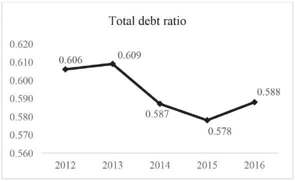
Figure 1 shows the historical total debt ratio from 2012 to 2016 of the Ecuadorian companies.
Source: Superintendence of Companies, Securities and Insurance.
Figure 1 Total debt ratio of all Ecuadorian companies.
It is observed that in all the time between, the ratio did not have a great variation. In 2012, for example, 60.6% of corporate assets were financed by debt, while in 2015 it reached a minimum level of 57.8% and ended up rebounding to 58.8%. Ecuador, being a country with a heavy dependence on oil revenues, experienced a severe blow to its economy by the fall in crude oil prices between 2014 and 2015. In fact, according to reports from the Central Bank of Ecuador, the volume of credit granted by financial institutions had a drastic reduction between 2015 and 2016.
The values obtained from the descriptive statistics are shown in the following table;
Table 2 Descriptive statistics of the variables studied.
| Variable | Obs. | Media | Desv. Est | Min | Max |
| RD | 1,520 | 0.5749 | 0.2609 | 0.0001 | 1.9257 |
| RENT | 1,520 | 0.0871 | 0.1342 | -1.0697 | 0.9482 |
| TAM | 1,520 | 13.9179 | 1.7022 | 7.0244 | 19.3039 |
| EFND | 1,520 | 0.0386 | 0.0420 | 0.0001 | 0.5111 |
| TANG | 1,520 | 0.3482 | 0.2578 | 0.0000 | 0.9975 |
| LIQ | 1,520 | 4.6517 | 22.9721 | 0.0581 | 612.1120 |
| OC | 1,520 | 1.2610 | 209.1887 | -4926.3020 | 6050.3210 |
Source: own elaboration.
The total debt ratio (DR) indicates that 57.4% of the total assets of the companies under consideration are financed through debt, regardless of whether it is long or short term.
Profitability, measured by ROA, shows an average of 8.7% along with a standard deviation of 13.4%, indicating a large variation of returns on assets within the sample. The presence of tax shields not generated by debt represents only 3.8% of balance sheet expenditures, with a standard deviation of 4.2%. Tangibility, on the other hand, indicates that on average companies have 34.8% of net fixed assets in their balance sheets, with a standard deviation of 25.8%. Regarding liquidity, the average indicates that current liabilities are covered 4.7 times by current liabilities, with a standard deviation of 22.9. Finally, the GO (growth opportunities) variable indicates that, on average, for every 1% increase in the total assets of the companies, their sales increase 1.3 times.
Table 3 shows the low correlation of the variables with each other and with the debt ratio.
Table 3 Pearson correlation coefficient matrix.
| RD | RENT | TAM | EFND | TANG | LIQ | OC | |
| RD | 1.0000 | ||||||
| RENT | -0.3194 | 1.0000 | |||||
| TAM | 0.1640 | 0.1200 | 1.0000 | ||||
| EFND | -0.0280 | 0.0723 | -0.1012 | 1.0000 | |||
| TANG | -0.1125 | -0.1385 | -0.0123 | 0.3355 | 1.0000 | ||
| LIQ | -0.1925 | 0.0282 | -0.1923 | -0.0442 | -0.0375 | 1.0000 | |
| OC | 0.0122 | 0.0093 | 0.0272 | 0.0415 | 0.0514 | -0.1003 | 1.0000 |
Source: own elaboration.
It can be observed that the correlation between the TSNGD and the TANG is the highest positive of all. This is explained by the fact that the more net fixed assets a company owns, the greater the expense for depreciation of those assets and, consequently, the TSNGD measure increases simultaneously with TANG. On the contrary, the variables DR and PROF show a negative correlation; this could be explained by the fact that a higher level of debt increases interest payments, reducing pre-tax profits.
After the correlation results, Table 4 shows the Variance Inflation Factor for each variable. Remarkably, they are at low levels-1.09 on average-indicating a low correlation between the variables. Thanks to this test it can be stated that there is no significant problem of multicollinearity.
Table 4 Variance Inflation Factor
| Variable | FIV | 1/FIV |
| EFND | 1.17 | 0.85673 |
| TANG | 1.17 | 0.85752 |
| TAM | 1.07 | 0.93117 |
| RENT | 1.06 | 0.94434 |
| LIQ | 1.06 | 0.94705 |
| OC | 1.01 | 0.98682 |
| FIV prom | 1.09 |
Based on the above data, the Ordinary Least Squares (OLS) model has been tested and the results are presented in the following Table
Table 5 Results of the OLS model.
| R^2 | 0.1968 | F | 61.7753 | |
| R^2 tight | 0.1936 | Prob > F | 0.0000 | |
| Typical error | 0.2343 | SSE | 83.0256 | |
| Observations | 1520 | SSR | 20.3394 | |
| Variables | Coef. | standard error | t | P>t |
| RENT | -0.7181 | 0.0461 | -15.58 | 0.0000 |
| TAM | 0.0283 | 0.0037 | 7.73 | 0.0000 |
| EFND | 0.4672 | 0.1547 | 3.02 | 0.0030 |
| TANG | -0.1946 | 0.0252 | -7.73 | 0.0000 |
| LIQ | -0.0017 | 0.0003 | -6.35 | 0.0000 |
| OC | 0.0000 | 0.0000 | 0.1 | 0.9210 |
| Interception | 0.3013 | 0.0523 | 5.76 | 0.0000 |
Source: own elaboration.
Before selecting the model that best explains the relationships between the variables, the Hausman test was carried out.
Table 6 indicates a p-value = 0.0034 that prevents rejection of the null hypothesis, which states that there is no correlation between individual effects and explanatory variables. Therefore, it was decided that the appropriate model was the fixed effects model.
Table 6 Hausman test for fixed effects and random effects models.
| Variables | E. Fixed | E. Random | Diferencia | Err. Std. |
| Coef | Coef | (ef-ea) | ||
| RENT | -0.50998 | -0.53835 | 0.02837 | 0.01278 |
| TAM | 0.03007 | 0.03005 | 0.00003 | 0.00831 |
| EFND | 0.46788 | 0.45842 | 0.00946 | 0.44423 |
| TANG | -0.10648 | -0.13130 | 0.02482 | 0.01614 |
| LIQ | -0.00061 | -0.00077 | 0.00017 | 0.00006 |
| OC | 0.00001 | 0.00001 | 0.00000 | 0.00000 |
| _Const | 0.22253 | 0.23513 | ||
| Hausman | 17.690 | |||
| p-value | 0.0034 |
Source: own elaboration.
According to the results of the Fixed Effects Model, Table 7, at a 5% level of significance the variables of profitability, size, tax shields not generated by debt, tangibility of assets, and liquidity are highly significant. Only the GO (growth opportunities) variable appears to be highly non-significant under the same level of significance.
Table 7 Fixed Effects Model.
| R^2 | 0.1830 | F | 38.09 |
| Corr (Ui_Xb) | 0.1334 | Prob > F | 0.0000 |
| Observations | 1520 | Group | 304 |
| Variables | Coef. | P > | t | | |
| RENT | -0.5100 | 0.0000 | |
| TAM | 0.0301 | 0.0030 | |
| EFND | 0.4679 | 0.0010 | |
| TANG | -0.1065 | 0.0010 | |
| LIQ | -0.0006 | 0.0050 | |
| OC | 0.0000 | 0.4740 | |
| _cons | 0.2225 | 0.1190 |
Source: own elaboration.
The value of R2 is 0.1968 and indicates that only 19.6% of the variation of total indebtedness (DR) is explained by the effect of independent variables.
Table 8 shows the results obtained from the Random Effects Model, which measures the effect of each explanatory variable with respect to dependent variable, debt ratio, with a statistical significance of each of them in each model. An error level of 5% (0.05) has been considered, together with a confidence level of 95%.
Table 8 Predictions of each theory and the results of the fixed effects model.
| Variable | Theory | ||
| TEE | TJF | Modelo | |
| Prediction | Prediction | Sign | |
| Profitability | + | - | -* |
| Size | + | - | +* |
| Tax shields | - | n/a | +* |
| Tangibility | + | - | -* |
| Liquidity | + | - | -* |
| Growth opportunities | - | + | + |
Source: own elaboration.
Empirical results suggest that profitability has a negative and highly significant relationship to the level of corporate debt. This result is consistent with what is expected only under the POT, but not under the TOT. The POT assumes that companies prefer to use their own resources rather than borrow, so the more profitable the company, the less debt it will use as a financial resource. The result obtained is similar to that of other researches (Serrasqueiro, Matias, & Salsa, 2016; Huang & Song, 2006; Chen & Chen, 2011; Saeedi & Mahmoodi, 2009; Acaravci, 2016; Tanaka, 2008; Khrawish & Khraiwesh, 2010; Booth, Aivazian, Demirguc-Kunt, & Maksimovic, 2001; Eriotis, Frangouli, & Ventoura-Neokosmides, 2011). Hypothesis H2 is accepted.
According to the TOT, size has a positive relationship with indebtedness. The results of the model show a positive and highly significant relationship between both variables, thus verifying the hypothesis of the TOT with respect to this relationship. The explanation, according to the theory, is that the larger the company, the more diversified it is and the lower the risk of a) bankruptcy and 2) income volatility. These two qualities motivate directors to borrow at higher levels and relax the demands of the creditors. This result only supports the prediction of the TOT, not the POT. The result of this study is similar to that of other authors (Acedo, Alútiz, & Ruiz, 2012; Kouki & Said, 2012; Eriotis, Vasiliou, & Ventoura-Neokosmidi, 2007; Khrawish & Khraiwesh, 2010; Serrasqueiro & Caetano, 2015). Hypothesis H3 is accepted.
The TOT suggests a negative relationship between the level of debt and the TSNGD. The results of the model show a positive and significant relationship between the variables. The explanation for this could be that companies use their fixed assets as collateral for debt, which would increase the expense of depreciation of assets at the time of acquisition, and the level of debt. This result does not support the prediction of the TOT. Other studies showed similar results to this one (Serrasqueiro, Matias, & Salsa, 2016; Serrasqueiro & Caetano, 2015; DeAngelo & Masulis, 1980). Hypothesis H5 is accepted.
Both the TOT and the POT predict a positive relationship between asset tangibility and level of debt. Such a prediction would be based on the fact that companies offer their tangible assets as debt collateral, so the more tangible assets the company has, the higher its level of debt. The results of the model suggest the opposite, that is, both variables have a negative relationship, indicating that the level of debt should not necessarily increase in light of the presence of a large quantity of tangible assets. This result is similar to other researches (Serrasqueiro, Matias, & Salsa, 2016; Kouki & Said, 2012; Saeedi & Mahmoodi, 2009; Acaravci, 2016; Booth, Aivazian, Demirguc-Kunt, & Maksimovic, 2001). One factor that could cause this negative relationship would be that tangible assets do not have a high market value, which would discourage creditors from accepting them as collateral for debt. Hypothesis H7 is accepted.
The model suggests a significant negative relationship between liquidity and the debt ratio. This result is consistent with the predictions in the POT, but not with the TOT. This result is similar to that of other researches (Serrasqueiro, Matias, & Salsa, 2016; Saeedi & Mahmoodi, 2009; Eriotis, Vasiliou, & Ventoura-Neokosmidi, 2007). The logic behind this relationship is that companies prefer to use retained earnings as a way of financing themselves. This result is very consistent with what was found in a study of SMEs in Guayaquil: almost half of the directors of these companies indicated that the main problem at the time of financing is the cost of financing, i.e. high interest rate on credit (Moran, Jácome, & Rodríguez, 2017). Hypothesis H10 is accepted.
Lastly, the GO (growth opportunities) variable has no statistical significance in the model. This result confirms that the expected growth of companies, considered as an intangible asset, cannot be used as collateral for debt, which implies that the debt ratio is not affected.
Conclusions
This empirical study has explored the determinants of the capital structure of 304 Guayaquil companies during the period of 2012-2016 using a panel data structure and analyzing it using a Fixed Effects Model.
The results indicate that there is a negative relationship between profitability, tangibility, and liquidity with respect to corporate indebtedness. Conversely, size and tax shields not generated by debt have a significantly positive relationship with indebtedness. Only the variable “growth opportunities” turned out not to have any statistical importance on the level of debt.
The evidence of the explanatory power of the Trade-off Theory of Capital Structure regarding the type of financing preferred by Guayaquil companies is weak. This theory could only predict the relationship of a determinant with the level of debt with the size of the company. In other words, the results of the model suggest a significant and positive relationship between the size and level of debt. On the other hand, the Picking Order Theory was able to predict almost accurately the relationship of each factor and its relationship to the level of debt and the choice of financing. Consequently, it better predicts the financial behavior of the sample. The latter correctly predicted the relationships of profitability, tangibility, liquidity, and growth opportunities (although the latter was not statistically significant), but not the relationship of company size to indebtedness. The results of the model agree with three predictions of this theory: a negative and significant correlation between profitability, liquidity, and the level of debt; and positive, but not significant, between growth opportunities and the level of debt. The results are consistent with four of the five predictions of this theory.
The reason why there is a negative relationship between profitability, tangibility, and liquidity, and a positive relationship between size and tax shields not generated by debt against the level of debt is as follows: companies prefer to use their own resources to finance themselves, so the more profitable and liquid the company, the less debt it requires. With respect to tangibility, companies with lower levels of fixed assets have a higher level of indebtedness. These companies are presumed to 1) provide current assets as collateral and/or 2) use short-term debt as a financing option.
Concerning the size and tax shields not generated by debt, it is presumed that larger companies obtain greater credits thanks to the low risk of bankruptcy and non-payment of the same, by having a more diversified business than a smaller company. While for tax shields not generated by debt, it is presumed that companies do use debt to take advantage of tax deductions due to interest expenditure.
This leads to the conclusion that a company affiliated to CAPIG definitively prefers to finance itself rather than contract debt with banks or issue debt instruments. These results are consistent with those obtained from Tenjo, López & Zamudio (2006) for Colombian companies; Paredes, Ángeles, & Flores (2016) for companies in five Latin countries; Booth, Aivazian, Demirguc-Kunt, & Maksimovic (2001) for companies in ten developing countries; and Acaravci (2016) for Turkish companies.
According to a study conducted by the Universidad de Especialidades Espiritu Santo, presented in 2017, 90% of existing Ecuadorian companies are family-owned. This means that it is very likely that both shareholders and directors are related to each other, leaving little room for investors outside the family.
The cost of debt could be an important aspect to consider in order to better understand why companies prefer to finance themselves rather than get into debt. In Ecuador, the interest rate for business loans is in the range of 7-10%5 per annum on average; Colombia, 8-12%6; while in countries such as Chile and Perú it is 5-7%7 and 3-5%8, respectively.
Future lines of research should integrate the historical interest rate into the models to estimate the effect they have on the choice of financing by the companies. In addition, it would be enriching to know the determinants of the capital structure by sector and industries of the economy, also adding a variable that segregates companies among family or non-family, so as to have more precise estimates of corporate financing preferences with a wide level of detail.
REFERENCES
Acaravci, S. (2016). The Determinants of Capital Structure: Evidence from the Turkish Manufacturing Sector. International Journal of Economics and Financial Issues, 5(1), 158 - 171. [ Links ]
Acedo, M. A., Alútiz, A., & Ruiz, F. (2012). Factores Determinantes de la Estructura de Capital de las Empresas Españolas. Tribuna de Economía, 868, 155-172. [ Links ]
Berkovitch, E., Israel, R., & Spiegel, Y. (2000). Managerial Compensation and Capital Structure. Journal of Economics & Management Strategy, 9(4), 549-584. doi:https://doi.org/10.2139/ssrn.142951 [ Links ]
Booth, L., Aivazian, V., Demirguc-Kunt, A., & Maksimovic, V. (2001). Capital Structure in Developing Countries. The Journal of Finance,56(1) 87-130. doi:https://doi.org/10.1111/0022-1082.00320 [ Links ]
Bradley, M., Jarrell, G., & Kim, H. (1984). On the Existence of an Optimal Capital Structure: Theory and Evidence. The Journal of Finance, 39(3), 857-878. doi:https://doi.org/10.2307/2327950 [ Links ]
Chen, L.-J., & Chen, S.-Y. (2011). How the Pecking-Order Theory Explain Capital Structure. Journal of International Management Studies, 1-9. [ Links ]
DeAngelo, H., & Masulis, R. (1980). Optimal Capital Structure Under Corporate and Personal Taxation. Journal of Financial Economic, 8(1), 3-29. doi:https://doi.org/10.1016/0304-405x(80)90019-7 [ Links ]
Eriotis, N., Vasiliou, D., & Ventoura-Neokosmidi, Z. (2007). How firm characteristics affect capital structure: an empirical study. Managerial Finance, 33(5), 321-331. doi: https://doi.org/10.1108/03074350710739605 [ Links ]
Fama, E., & French, K. (2002). Testing Trade-off and Pecking Order predictions about dividend and debt. The Review of Financial Studies, 15 (1) 1-33. doi:https://doi.org/10.1093/rfs/15.1.1 [ Links ]
Ferrer, M., & Tanaka, Á. (2009). Las PyMES y las teorías modernas sobre estructura de capital. Compendium (22), 65-83. [ Links ]
Franco, G., López, L., & Muñoz, G. (2010). Determinantes de la estructura de capital de las grandes empresas manufactureras en Uruguay. Econoquantun, 5, 4-25. [ Links ]
Frank, M., & Goyal, V. (2009). Capital Structure Decisions: Which Factors Are Reliably Important? Financial Management, 38(1), 1-37. doi:http://dx.doi.org/10.1111/j.1755-053X.2009.01026.x [ Links ]
Hernández, G., & Ríos, H. (2012). Determinantes de la estructura financiera en la industria manufacturera: la industria de alimentos. Análisis Económico, 27 (65), 101-121. [ Links ]
Huang, S., & Song, F. (2006). The Determinants of Capital Structure: Evidence from China. China economic review, 17 (1), 14-36. doi:https://dx.doi.org/10.2139/ssrn.320088 [ Links ]
Jorgensen, J., & Terra, P. (2003). Determinants of capital structure in Latinamerica: The role of firm-specific and macroeconomic factors. Annual Meeting of Multinational Finance Society. [ Links ]
Khrawish, H., & Khraiwesh, A. (2010). The Determinants of the Capital Structure: Evidence from Jordanian Industrial Companies. Economics and Administration, 24(1), 173-196. doi:https://doi.org/10.4197/Eco.24-1.5 . [ Links ]
Kolay, M., Schallheim, J., & Wells, K. (2013). A New Measure for Non-debt Tax Shields and the Impact on Debt Policy. University of Utah Working Paper. [ Links ]
Kouki, M., & Said, H. (2012). Capital Structure Determinants: New Evidence from French Panel Data. International Journal of Business and Management, 7(1). doi: http://dx.doi.org/10.5539/ijbm.v7n1p214 [ Links ]
Labra, R., & Torrecillas, C. (2014). Guía cero para datos de panel: un enfoque práctico. Madrid: UAM-Accenture. [ Links ]
Leland, H. (1998). Agency Costs, Risk Management, and Capital Structure. The Journal of Finance, 53 (4), 1213-1243. doi:http://dx.doi.org/10.1111/0022-1082.00051 [ Links ]
Miller, M. (1977). Debt and Taxes. The Journal of Finance, 32 (2), 261-275. doi:http://dx.doi.org/10.1111/j.1540-6261.1977.tb03267.x [ Links ]
Modigliani, F., & Miller, M. (1958). The Cost of Capital, Corporation Finance and the Theory of Investment. The American Economic Review, 48 (3), 261-297. [ Links ]
Modigliani, F., & Miller, M. (1963). Corporate Income Taxes and the Cost of Capital: A Correction. The American Economic Review, 53(3), 433-443. [ Links ]
Moran, C., Jácome, D., & Rodríguez, L. (2017). Emisiones sindicadas de obligaciones como alternativa de financia-miento para las PyME del sector metalmecánico en Guayaquil. Revista Ciencia UNEMI, 10(22), 11-19. [ Links ]
Mou, W. (2011). The Determinants of Capital Structure in Chinese Listed Companies. Masters thesis. Universiti Utara Malaysia. [ Links ]
Myers, S. (1977). Determinants of Corporate Borrowing. Journal of Finance, 5(2), 147-175. doi:https://doi.org/10.1016/0304-405X(77)90015-0 [ Links ]
Myers, S. (1984). The Capital Structure Puzzle. The Journal of Finance, 39(3). doi: http://dx.doi.org/10.1111/j.1540-6261.1984.tb03646.x [ Links ]
Myers, S., & Majluf, N. (1984). Corporate Financing and Investment Decisions when Firms Have Information The Investor do not Have. Journal of Financial Economics, 13(2). doi:https://doi.org/10.1016/0304-405X(84)90023-0 [ Links ]
Padilla Ospina, A., Rivera Godoy, J., & Ospina Holguin, J. (2015). Determinantes de la estructura de capital de las mipymes del sector real participantes del Premio Innova 2007-2011. Revista Finanzas y Política Económica, 7 (2), 359-380. [ Links ]
Paredes, A., Ángeles, G., & Flores, M. (2016). Determinants of leverage in mining companies, empirical evidence for Latin American countries. Contaduría y Administración, 61 (1), 26-40. [ Links ]
Rajan, R., & Zingales, L. (1995). What Do We Know about Capital Structure? Some evidence from international data. The Journal of Finance, 50 (5), 1421-1460. [ Links ]
Saeedi, A., & Mahmoodi, I. (2009). The Determinants of Capital Structure: Evidence from an Emerging Market. Recent Advances in Business Administration, 17(1/2), 13-18. doi:https://doi.org/10.1108/10569210710774730 [ Links ]
Serrasqueiro, Z., & Caetano, A. (2015). Trade-Off Theory versus Pecking Order Theory: capital structure decisions in a peripheral region of Portugal. Journal of Business Economics and Management, 16 (2), 445-466. doi:https://doi.org/10.3846/16111699.2012.744344 [ Links ]
Serrasqueiro, Z., Matias, F., & Salsa, L. (2016). Determinants of capital structure: New evidence from Portuguese small firms. Dos Algarves: A Multidisciplinary e-Journal, 28, 13-28. doi:http://dx.doi.org/10.18089/DAMeJ.2016.28.1.2 [ Links ]
Sheikh, N., & Wang, Z. (2011). Determinants of capital structure: an empirical study of firms in manufacturing industry of Pakistan. Managerial Finance, 37(2), 117-133. doi:https://doi.org/10.1108/03074351111103668 [ Links ]
Sultan, A., & Adam, M. (2015). The Effect of Capital Structure on Profitability: An Empirical Analysis of Listed Firms in Iraq. European Journal of Accounting, Auditing and Finance Research, 3(2), 61-78. [ Links ]
Tanaka, Á. (2008). Comportamiento de la Estructura Financiera en un Grupo de Empresas Españolas previo a la participación de capital de riesgo. Documentos de trabajo en finanzas de empresas(2). [ Links ]
Tenjo, F., López, E., & Zamudio, N. (2006). Determinantes de la estructura de capital de las empresas colombianas: 1996-2002. Coyuntura Económica, XXXVI(1), 117-147. [ Links ]
Titman, S., & Wessels, R. (1988). The Determinants of Capital Structure Choice. The Journal of Finance, 43(1), 1-19. doi:http://dx.doi.org/10.1111/j.1540-6261.1988.tb02585.x [ Links ]
Warner, J. (1977). Bankruptcy Costs: Some Evidence. The Journal of Finance, 32(2), 337-347. doi:http://dx.doi.org/10.1111/j.1540-6261.1977.tb03274.x [ Links ]
1 http://www.capig.org.ec/. This institution is made up of companies that mostly belong to the SME category. It has 521 associates, of which 433 are incorporated companies and the rest are natural persons.
2Available on http://www.supercias.gob.ec
Received: December 20, 2017; Accepted: May 21, 2018
 Este es un artículo publicado en acceso abierto bajo una licencia Creative Commons
