


 nueva página del texto (beta)
 Inglés (pdf)
 Artículo en XML
 Referencias del artículo
 Enviar artículo por email
 Citado por SciELO
  Similares en
SciELO
Similares en
SciELO 
 Permalink
1. INTRODUCTION
Chromospheric activity is an interaction between the magnetic field and the plasma. Solar spots and flares are well-known examples of this phenomenon. The oldest records of sunspots are found in Chinese records dating back 2000 years (Clark & Stephenson 1978; Wittmann & Xu 1987). For the first time in the literature, Kron (1950) discovered that UV Ceti stars also exhibit spot activity. Kron (1950) detected the sinus-like variations in the light curve of an eclipsing binary YY Gem, and then Kunkel (1975) called this event the BY Dra Syndrome, in which the variation is caused by a heterogeneous temperature distribution on the stellar surface.
Berdyugina & Usoskin (2003) found on the
solar surface two active longitudes separated by 180
A flare event is a consequence of magnetic reconnection in the outer convective envelope of the star (Pettersen 1989). Flare activity was first detected on the solar surface by Carrington (1859) and Hodgson (1859). UV Ceti is the first star on which flare activity was detected. According to Skumanich’s law, the younger stars have a higher rotational velocity, which causes the activity level to increase (Skumanich 1972; Marcy & Chen 1992). This is the reason why the dwarfs found in open clusters mostly show flare activity (Mirzoian 1990; Pigatto 1990). This is also the reason why the number of UV Ceti type stars decreases with increasing cluster age (Marcy & Chen 1992; Pettersen 1991; Stauffer 1991).
The mass loss rate increases with increasing flare activity level. The solar
mass-loss rate is known to be
Among the parameters of flares, energy is an important one. There is a marked difference between the flare energies obtained from stars of different spectral types. The energies measured from tworibbon flares generally have a level between 1030 and 1031 ergs (Gershberg 2005; Benz 2008). RS CVn binaries have many flares with an energy level of 1031 erg (Haisch et al. 1991). According to the longterm observations, the energies of the flares detected from dMe stars range from 1028 to 1034 erg (Gershberg 2005). The flare energies measured from the members of the Pleiades cluster and Orion Association can reach 1036 erg (Gershberg & Shakhovskaia 1983). Although the observations show that there are significant differences between solar and stellar flares when it comes to mass-loss ratio or flare energy levels, stellar flare events are still explained by the solar flare processes. In the studies such as Aschwanden et al. (2017); Gershberg (2005) and Hudson & Khan (1996), it is argued that magnetic reconnection processes are the dominant energy source in flare events.
In this study, both flare and spot activities of KOI 6652 (KIC 6044064) are examined. The results are compared with the chromospheric activity behaviour of UV Ceti-type stars.
The JHK brightnesses of the system are given as 13
m
.485, 12
m
.976, 12
m
.853 in the 2MASS All-Sky Survey Catalogue, respectively (Cutri et al. 2003). A detailed light curve
analysis of the system cannot be found in the literature. However, the temperatures
of the components were estimated by Kjurkchieva et
al. (2017) to be 5095 K for the primary component and 3032 K for the
secondary component. In the same study, the mass ratio (
2. DATA AND ANALYSES
The Kepler Space Telescope, which has observed more than 150,000 sources, was launched for the discovery of exoplanets (Borucki et al. 2010; Koch et al. 2010; Caldwell et al. 2010). The Kepler observations are the most sensitive photometric data ever obtained (Jenkins et al. 2010a,b). In addition to exoplanets, many variable stars have also been discovered (Slawson et al. 2011; Matijevič et al. 2012). There are many single and binary stars exhibiting spot and flare activity among them (Balona 2015). For the target, photometric data were taken from the Kepler Database (Slawson et al. 2011; Matijevič et al. 2012).
Long cadence (hereafter LC) data were used in all analyses. KIC 6044064 was observed for 1384.254 days, from JD 2454964.512414 to JD 2456424.001369, with some technical interruptions. After removing observations with large errors due to the technical problems, the phases were calculated using the ephemerides from the Kepler Mission database. The data were arranged into appropriate formats for the analysis of different variations such as flare activity, spot activity and (O−C) variations. All the available long cadence data of KIC 6044064 are shown in Figure 1.
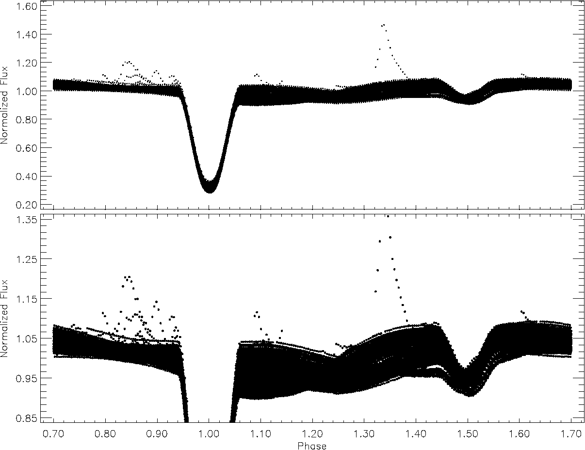
Fig. 1 The light variation obtained from the long cadence data taken from the Kepler database is plotted versus the phase depending on the orbital period.
2.1. Orbital Period Variation
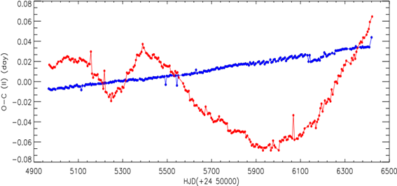
The minima times of the system were obtained without correction from the LC data. The minima times were calculated using a script depending on the method described by Kwee & van Woerden (1956). Each minimum in the light curves was fitted separately using the high-order spline functions. Using these fits, a total of 525 minima times were obtained. 264 of them were computed from the primary minima, while 261 of them were calculated from the secondary minima. The deviations between observed and calculated minima times were calculated as (O − C) differences. We show these differences by the term of (O − C) I . We noticed that the (O − C) differences show a linear trend due to the incorrect orbital period, which needs to be adjusted. Using the least squares method, we modelled the distribution of the (O−C) differences versus the observation time. To remove the linear trend of the distribution, a linear correction given by Equation (1) was applied to the (O − C) distribution.
where the term HJD (Hel.) is the Heliocentric Julian Day, while the first term on
the right side of the equation is the epoch, and the second term is the orbital
period of the system. The number in parenthesis seen in the equation is the
error of each term on the right side. The parameter
In the last step we computed the deviations between the linear fit and the (O −C) I differences; we call these the secondary residuals (O−C) II . In Figure 2, an interesting variation is seen in the plane of (O−C) II versus time. The (O−C) II residuals vary in time, but in different directions. The (O − C) II residuals of the primary minima still vary in a linear trend, while those of the secondary minima vary in a sinusoidal form. As indicated by Tran et al. (2013) and Balaji et al. (2015), the secondary minima are strongly affected by the position of the spotted area and its movement on the component, while the residuals of the primary minima are not affected as much.
2.2. Light Curve Analyses
To obtain an acceptable solution from the light curve analyses of the LC data, the distortion caused by the flare activity was removed from the light curve. Finding two consecutive cycles that were least affected by the sinusoidal variation, we averaged their data with a phase interval of 0.005. Using the PHOEBE V.0.32 software (Prša & Zwitter 2005), the light curve analysis was performed for these average data, shown by the filled black circles in Figure 3. The method used in the PHOEBE V.0.32 software is based on the 2015 version of Wilson-Devinney Code (Wilson & Van Hamme 2014). Several modes were first tried in the light curve analysis. The astrophysical and statistically acceptable solution was obtained in the detached mode, known as Mode 2.

Fig. 3 The light curve obtained by using the data averaged with the interval of 0.005 and the synthetic light curve are shown. In the figure, the filled circles represent the observations, while the red line represents the synthetic light curve. The color figure can be viewed online.
There are several studies in the literature on the components of KIC 6044064. The
temperatures of the primary and secondary components were given as 5095 K and
3032 K by Kjurkchieva et al. (2017),
respectively. However, the initial analyses did not yield a statistically
acceptable solution by taking these values. Because of this, using the
calibrations given by Tokunaga (2000), we
calculated the de-reddened colours from the infrared (H −
K) and (J−H) color
indexes given by Cutri et al. (2003) and
then we calculated the temperature as 5375 K from these values. In the light
curve analysis, the temperature of the secondary component was taken as a free
parameter, while the temperature of the primary component was taken as 5375 K.
The values for the albedos (A
1, A
2) and the gravity darkening coefficients (g
1, g
2) were determined according to convective stars for both components
(Lucy 1967; Ruciński 1969). In addition, the linear limb-darkening
coefficients (x
1, x
2) were taken from van Hamme
(1993). The dimensionless potentials (Ω1, Ω2),
the luminosity fraction of the primary component (L
1), and the inclination (i) of the system were taken
as adjustable parameters. The synthetic curve obtained from the light curve
analysis is shown in Figure 3, while the
solution parameters are tabulated in Table
1. The parameters
TABLE 1 The parameters obtained from the light curve analysis
| Parameter | Value |
|---|---|
|
|
0.948 |
|
|
83.04 |
|
|
5375 (fixed) |
|
|
3951 |
|
|
0.813 |
|
|
0.486 |
|
|
0.694 |
|
|
0.306 (fixed) |
|
|
0.32, 0.32 (fixed) |
|
|
0.50, 0.50 (fixed) |
|
|
0.61, 0.61 (fixed) |
|
|
0.736, 0.736 (fixed) |
|
|
0.5585 |
|
|
0.2515 |
|
|
1.186(fixed) |
|
|
2.513(fixed) |
|
|
0.611(fixed) |
|
|
0.550 (fixed) |
|
|
1.196 (fixed) |
|
|
0.297 (fixed) |
|
|
0.122 (fixed) |
|
|
1.350 (fixed) |
Using the calibrations given by Tokunaga
(2000), the spectral types of the components were determined as G7V +
K9V. Using the same calibrations, the mass of the primary component was
determined as 0.86
Considering the variation at out-of-eclipses, we notice that the system exhibits chromospheric activity. At this point, we compare the system with its analogues listed in the Gershberg et al. (1999) catalogue in the mass-radius plane, shown in Figure 4. The filled circles in the figure represent well-known active stars listed in the catalogue, while the line represents the zero-age main sequence (ZAMS) taken from Siess et al. (2000).
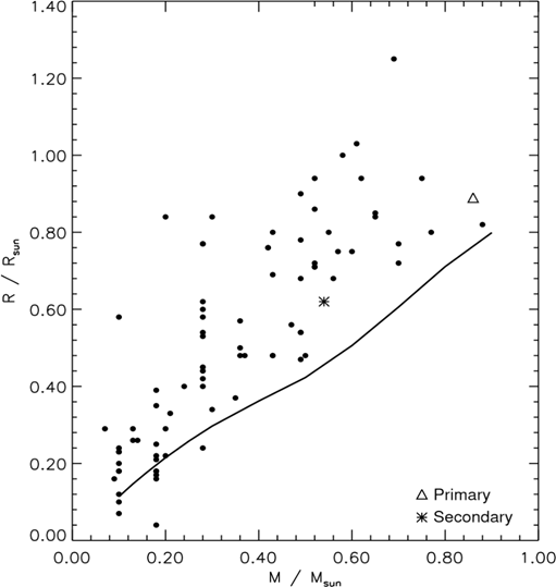
Fig. 4 The positions of the components are shown among UV Ceti type stars in the plane of mass-radius. The filled circles represent the target’s analogues listed by . The open triangle represents the primary component of KIC 6044064, while the asterisk shows the secondary component. The theoretical ZAMS model developed by is shown by the line.
2.3. Rotational Modulation and Stellar Spot Activity
It was seen that there is a remarkable sinusoidal variation excluding the flares at out-of-eclipses. Considering both the dominant flare activity and the components’ temperatures, it is clear that this variation should be a rotational modulation effect caused by the stellar spots. Examination of the consecutive cycles in the light curves, their minimum location, and level change over a few cycles, shows that the spotted area must evolve rapidly and move on the active component. Therefore, it is not possible to model all the light variation at once. For this reason, the data were split into several sets, considering the spot minimum phases with their levels for the consecutive cycles. Consequently, the entire LC data were divided into 11 subsets and modelled with two sinus waves. In this calculation, a Python script based on the Fourier method is used, and an example model is shown in Figure 5.
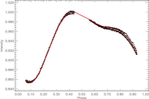
Fig. 5 The sinusoidal variation at out-of-eclipse between JD 2454982.188225 and JD 2454971.419273 is shown. In the figure, the black dots represent the observations, while the red line shows the model obtained by using the Fourier Method. The color figure can be viewed online.
The minima phases of the first sinusoidal variation show a temporal migration towards the early phases, while the minima phases of the second sinusoidal variation migrate in the same direction, but twice as fast as the previous one. This means that, at first sight, there are two spotted regions. However, we have noticed an interesting phenomenon that both the first and second sinusoidal variations should be caused by three separate spots in each area. Each of them separates into at least three spots because their minimum phases are separated into three parts by a phase interval of 0.33. These two distinct groups of spots and their migrations over time are shown in Figure 6.
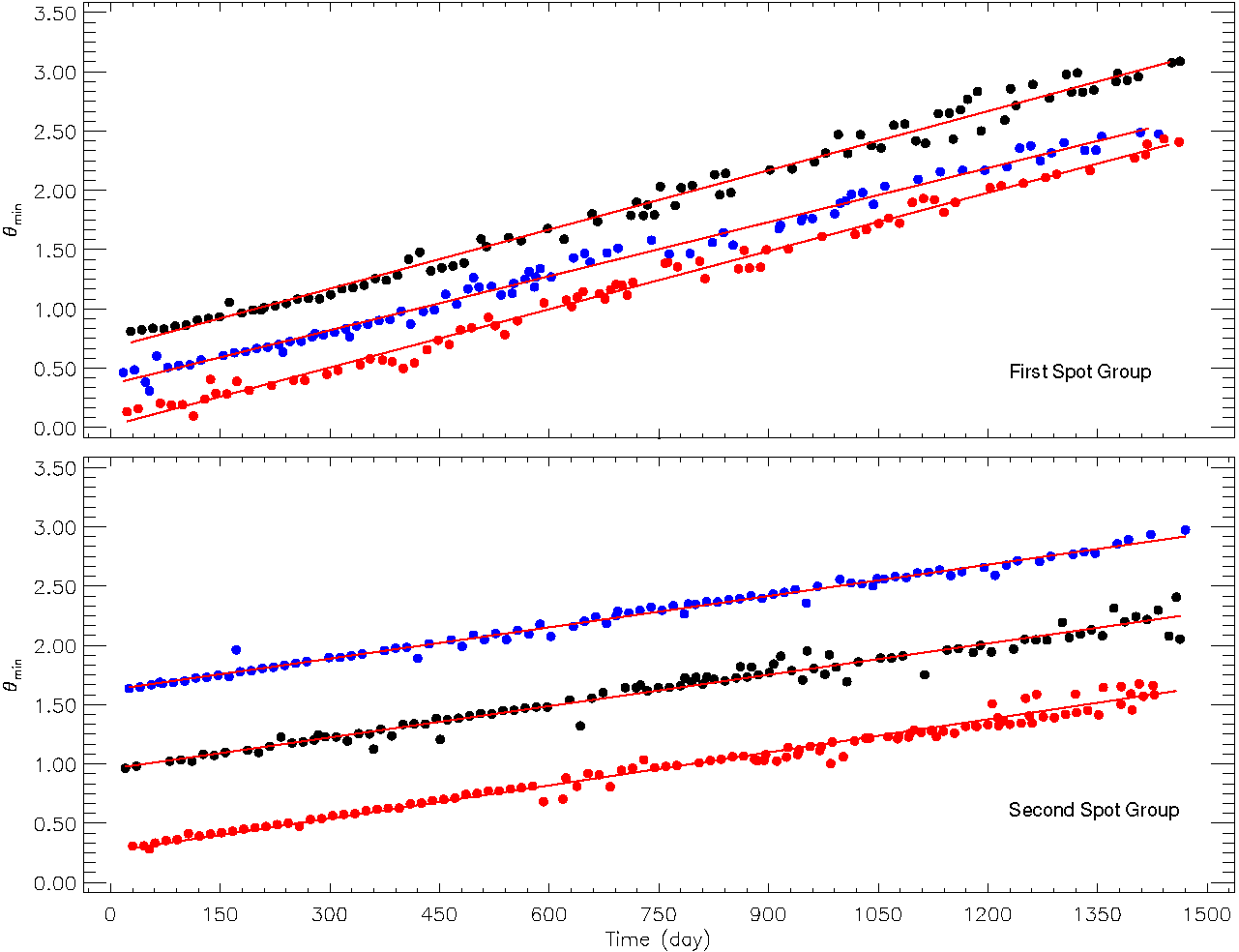
Fig. 6 The longitudinal spot migrations of the first group and their models are shown versus time in the upper panel, while they are shown for the second group in the lower panel. The filled black circles represent the first spot of both groups, the filled blue circles represent the second spot, while the filled red circles represent the third spot of the groups. The color figure can be viewed online.
As a result of the linear models created by the regression calculations with the least squares method, the spot migration periods of the first group were found to be 600.796±3.653 days (1.66±0.01 year), 657.726±3.653 days (1.80±0.01 year) and 610.665±7.305 days (1.67±0.02 year) from phase of 0.00 to 1.00, respectively. The spot migration periods of the second group were calculated as 1134.754±7.305 days (3.11±0.02 year), 1135.787±10.957 days (3.11±0.03 year) and 1106.286±7.305 days (3.03±0.02 year).
2.4. Flare Activity and OPEA Model
To study the flare behaviour of the system, all the variations apart from the flares are removed from the light curve. For this aim, we have used the synthetic curves derived by the light curve analysis for the geometrical effects and by the Fourier method for the sinusoidal variations.
In order to calculate the flare parameters, first of all, the flare beginning and end times need to be determined. Two examples are shown with their quiescent levels defined by the synthetic curves in Figure 7. In total, 44 flares with their parameters were determined. In the calculation, the equivalent durations were calculated using equation (2) defined by Gershberg (1972):
where
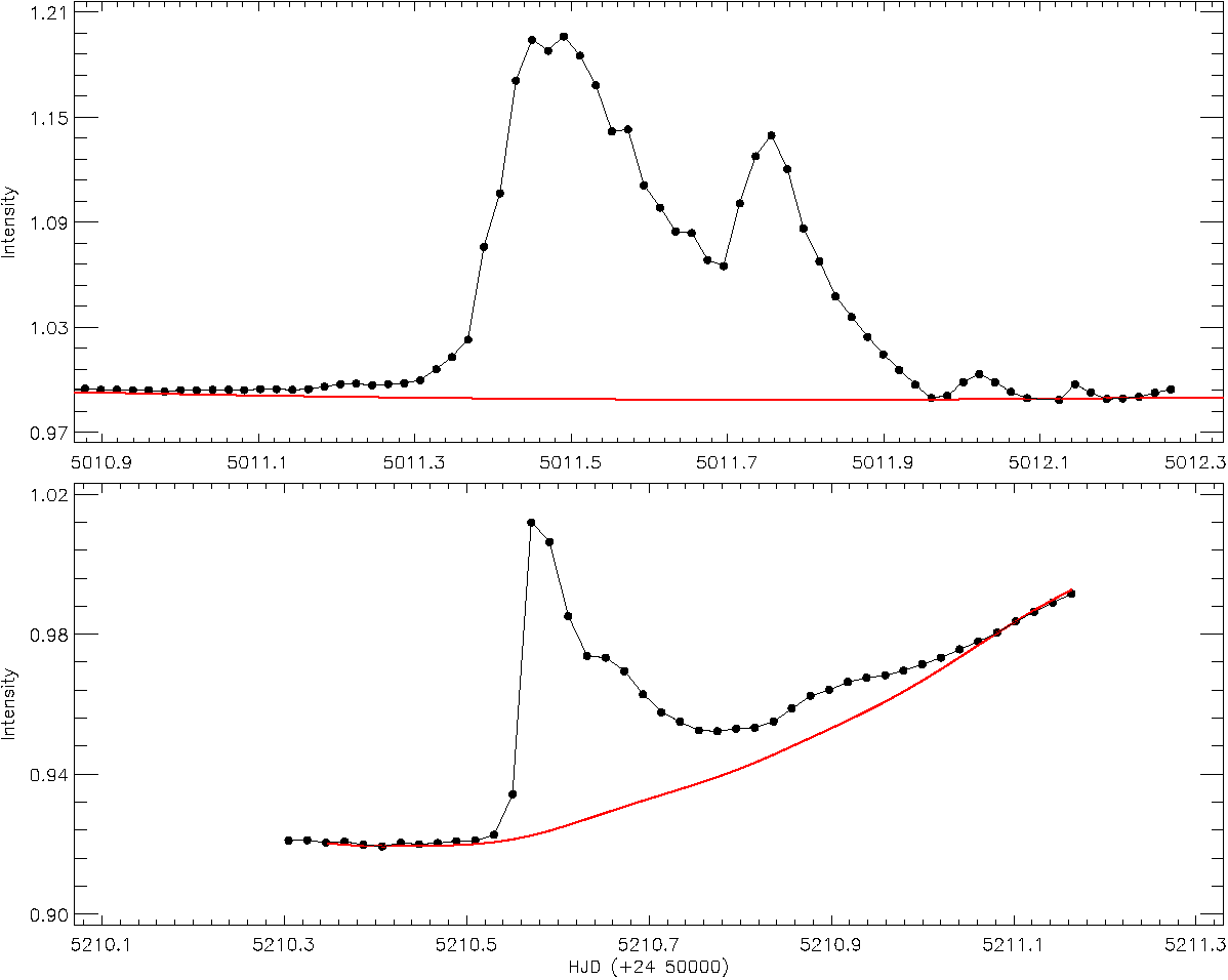
Fig. 7 Two flare examples detected from the target are shown. In the figure, the filled black circles show the observations, while the red lines show the quiescent levels defined by the Fourier method. The color figure can be viewed online.
Examining the relationships between the flare parameters, it is seen that the flare equivalent durations as a rule are distributed as a function of the total flare time. Following Dal & Evren (2010, 2011), regressions in SPSS V17.0 (Green et al. 1996) and GraphPad Prism V5.02 (Dawson & Trapp 2004) software were used to try to find the best function to model the distribution of flare equivalent durations via the flare total time on a logarithmic scale. In this step, the regression calculations showed that the best model is an exponential function known as the One Phase Exponential Association (hereafter OPEA) function. The OPEA is a special function with term Plateau defined by Equation (3) (Motulsky 2007; Spanier & Oldham 1987):
where the term y is the equivalent duration in the logarithmic scale; k is a constant and x is the total flare time, while y 0 is the theoretical flare equivalent duration obtained for the minimum total flare time (Dal & Evren 2011). The term Plateau defines the upper limit for the equivalent duration obtained from a given star. It means that the Plateau parameter gives a certain information about the maximum flare energy level of that star. In fact, the Plateau is the maximum equivalent duration. For this reason, the Plateau parameter is defined as the saturation level for the flare activity in the observed wavelength range for this particular target (Dal & Evren 2011). In order to derive the synthetic curve of the best model, we used the program GraphPad Prism V5.02, in which we used the least squares method for the non-linear regression calculations.
The obtained model is shown in Figure 8. The calculated model parameters are listed in Table 2. The span value listed in the table is the difference between Plateau and y 0 values. The half−life value is half of the first x value at which the maximum flare equivalent duration is reached. In other words, it is half of the total flare time at which the first highest flare energy is seen.
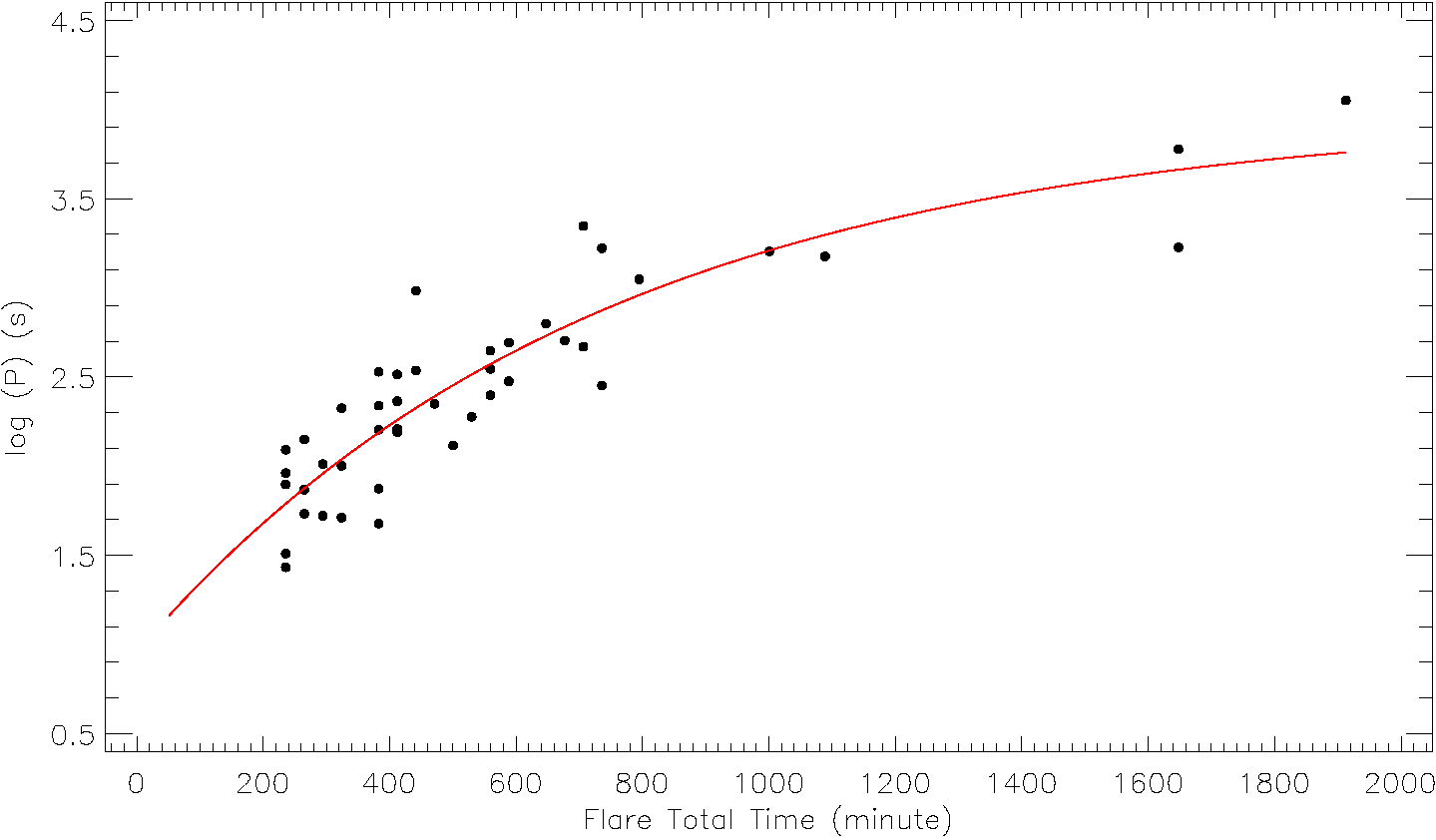
Fig. 8 The OPEA model obtained for 44 flares is shown. In the figure,
the filled circles represent the
TABLE 2 Parameters derived from the OPEA model
| Parameter | Values | 95 % Confidence Intervals |
|---|---|---|
| y0 | 0.958951 | 0.447653 to 1.47025 |
| Plateau | 3.9833 | 3.33968 to 4.62692 |
| K | 0.00002272 | 0.00001006 to 0.00003537 |
| Tau | 44022.7 | 28272.0 to 99399.2 |
| Half − time | 30514.2 | 19596.6 to 68898.3 |
| Span | 3.02435 | 2.53178 to 3.51692 |
| R2 | - | 0.85 |
* Using the least squares method.
KIC 6044064 was observed for a total of 1384.254 days (33222.09917 hours). From these observations, 44 flares were detected. The phases of 44 flares were calculated depending on the orbital period of the system, and the flare phase distribution of 44 flares is shown in Figure 9. The sum of equivalent durations is 35519.622 seconds over all flares. Two separate flare frequencies, N 1 and N 2, have been defined in the literature by Ishida et al. (1991). These frequencies are given by equations (4, 5):
where
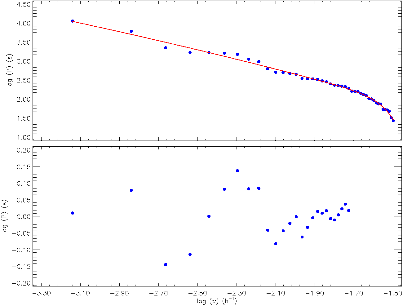
Fig. 9 The flare cumulative frequency distribution and its the exponential model derived for 44 flares are shown in the upper panel, while the residuals are shown in the bottom panel. The color figure can be viewed online.
We also computed the flare cumulative frequency distributions depending on each different energy limit. Gershberg (1972) defined the flare cumulative frequency distribution calculated separately for each different energy limit to reveal the character of the flare energy for given a star. Because of the above reasons, the flare equivalent durations is also used instead of the flare energy to compute the flare cumulative frequencies in this study. The obtained flare cumulative frequency distributions are shown in Figure 9. As can be seen in the figure, the flare cumulative frequencies exhibit a distribution in the form of an exponential function. In fact, the least squares method showed that an exponential function seems to be the most appropriate function to fit these distributions; hence we modelled the distributions with the exponential function. The obtained exponential functions are represented by the red line in Figure 9.
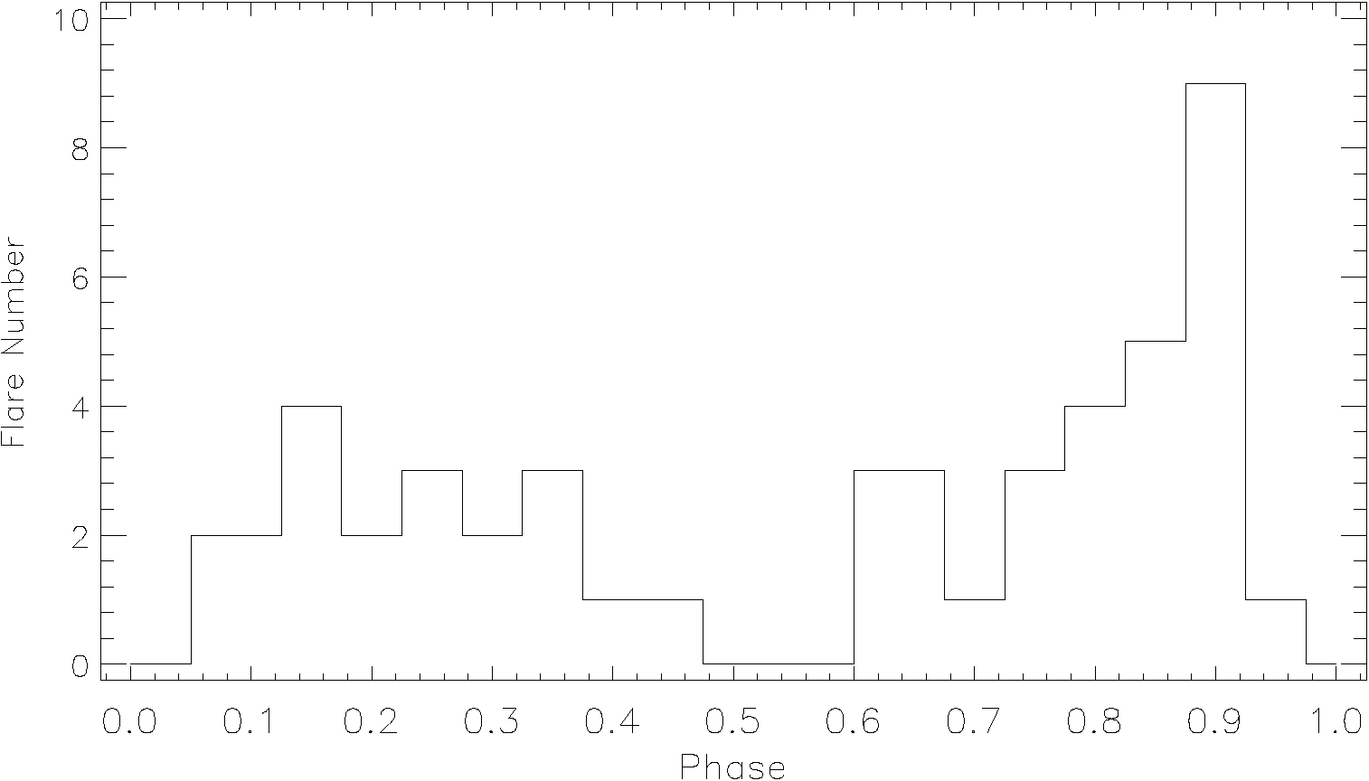
The standard models show that the flare energies emerge in the magnetic loops where the spots are located (Gershberg 2005; Benz 2008) at their foot points. Therefore, both the cool spots and the flares are expected to have the same phase distribution. To compare the phase distributions of these two activity structures obtained from KIC 6044064, the phase of each flare was calculated depending on the orbital period, then we obtained the total number of flares in each 0.05 phase interval. Their variation is shown in Figure 10.
3. RESULTS AND DISCUSSION
3.1. Orbital Period Variation
The (O − C) II residuals seem to vary in different ways. According to Tran et al. (2013) and Balaji et al. (2015), magnetic activity causes an affect on the variations of the minima times. The trends of primary and secondary minima time variations are expected to separate from each other due to the chromospheric activity. In the case of KIC 6044064, this effect reveals itself on the time variation of the secondary minima. The residuals of the secondary minima times exhibit a sinusoidal variation around zero with a large amplitude, although the primary minima times still show a linear trend. The linear corrections could not reduce the trend of the primary minimum residuals to zero, since the (O−C) I trend of the secondary minima times has a larger slope than that of the primary minima. It is more likely that the (O − C) II residuals of the primary minima should be a small part of a sinusoidal long-term oscillation due to the chromospheric activity.
3.2. Classification
The temperature of the primary component was found to be 5375 K, and that of the secondary was 3951 K. Thus, their spectral types were determined as G7V + K9V depending on the JHK brightness. Considering the temperatures and the estimated masses, we compared the system with its analogues. For this aim, we compared the components with other young flare stars on the mass-radius plane, which can be seen in Figure 4. It is expected that the flaring young stars listed by Gershberg et al. (1999) should be close to the ZAMS modelled by Siess et al. (2000). However, these stars appear to be somewhat evolved out of the main sequence, according to their positions on the mass-radius plane. It is possible that their calculated radii could be too large due to the high level chromospheric activity effects. Both the positions of the components in the mass-radius plane and the observed flare and spot activities indicate that KIC 6044064 should be an eclipsing binary system of the BY Dra type.
Both flare and stellar spot activities make it one of the stars having a high level of activity. The target has several rapidly evolving spots located on three active longitudes, which are separated from each other by 120 degrees inside two latitude bands.
In addition, the flare parameters are much higher than those obtained from all other chromospheric active stars. For example, KOI 6652 has a higher activity level than YY Gem, which has the same physical properties as KOI 6652 (Kochukhov & Shulyak 2019).
3.3. Spots
Indeed, KIC 6044064 has a high level of chromospheric activity. Apart from the flare activity, a sinusoidal variation is seen with a rapidly changing asymmetry at out-of-eclipses. This variation is caused by the evolving cool spots as well as their rapid longitudinal migration. There are two active longitudes on the solar surface, known as Carrington Coordinates, with a separation of 180◦ from each other. According to Bonomo & Lanza (2012), there are several active longitudes where stellar spots are formed. According to some authors, the active longitudes are stable structures with a constant rotational velocity relative to each other, although some authors claim that the active longitudes cannot have a constant rotational velocity, but have different rotational velocities relative to each other (Richardson 1947; Lopez Arroyo 1961; Stanek 1972; Bogart 1982). In the case of KIC 6044064, there are two different spot groups consisting of three spots located with a phase interval of 0.33 relative to each other. The phase interval of 0.33 corresponds to a longitude difference of 120◦. Both spotted areas on the stellar surface show migration in the same direction, but with different velocities. It is noteworthy here that each spot in a spot group shows the same longitudinal motion with a longitude interval of 120◦ at the same velocity. In particular, all three spots in the second group move at exactly the same velocity, so that their longitudinal positions on the stellar surface do not change at all relative to each other. For this reason, the slopes of the linear models of their longitudinal migrations have almost the same value up to the 4th digit.
As a result, the average migration period was found to be 623.063±4.870 days (1.71±0.01 year) for the first spot group, while it was 1125.514±7.305 days (3.08±0.02 year) for the second group. The values of the migration periods indicate that KIC 6044064 is generally a solar analogue. This is because the period of each group is in agreement with the periods between 1.5-3.0 years found for the active longitude migrations of the solar spots (Berdyugina & Usoskin 2003). The existence of fixed migrations and the migration period values can help us to configure the stellar surface. It is clear that both groups of spots should be located in the latitudes above the stellar co-rotation latitude, assuming that KIC 6044064 exhibits the standard differential rotation. The spots are located at a latitude where the rotation velocity is lower than the mean stellar rotation velocity, hence the minima of the sinusoidal variations migrate toward the increasing phases in the light curves. Moreover, the fact that the spots in each group move as if they were locked to each other indicates that the spots in each group should be located at nearly the same latitude. All these situations give the impression that there must be two spot-belts in two upper latitudes. The spotted regions should surround the stellar surface at two different latitudes above the co-rotation latitude, and different regions of the belts appear more active than other parts. Taking into account the average longitudinal migration periods, the trend of which is shown in the bottom panel of Figure 6, the second spot belt should be at higher latitudes. However, it should be noted here that these spot belts may not be located on the same component. This is because both components are most likely candidates for exhibiting chromospheric activity.
3.4. Flares
There should be three active longitudes on the secondary component, and the active longitudes are located with a longitude interval of 120 degrees. According to this scenario, it is possible that an observer can detect some flares from the longitudes per 120 degrees on the surface of the secondary component. In this case, we expect a nearly homogeneous phase distribution for the flares coming from the target. On the other hand, as can be seen in Figure 10, the total number of flares detected in each phase interval of 0.05 increases towards phases 0.15 and 0.85. The flare number starts to increase after phase 0.70 and decreases before phase 0.40. However, at phase 0.00, the flare number suddenly drops to almost zero. It is possible that during the primary minima, the active component is eclipsed by the other component towards the observer. Consequently, the flare frequency varies from one phase interval to the next; and it must reach a maximum between phases 0.85-0.15. Because of tidal effects, the flare occurring possibility on the surface facing the other component becomes higher than anywhere else on the surface, although the flares can occur anywhere on the stellar surface.
The Plateau value was determined to be 3.983 s over 44 flares detected from KIC 6044064. This value is so high that the secondary component must be compared with similar close binaries exhibiting flare activity. In this regard, we compared its flare nature with those obtained from KIC 9641031, KIC 9761199, KIC 11548140, KIC 12004834 (Yoldaş & Dal 2016, 2017b,a, 2019). This value was found to be 1.232 s for KIC 9641031, 1.951 s for KIC 9761199, 2.312 s for KIC 11548140 and 2.093 s for KIC 12004834. The plateau values of KIC 6044064 are much higher than those of its analogues. For this reason, it should be much more appropriate to compare the target with UV Ceti type single stars, which exhibit flare activity with high frequency and high energy level. Therefore, we compared the secondary component with EV Lac. The plateau value of EV Lac is 3.014 s (Dal & Evren 2011). It is clear that the plateau value of KIC 6044064 is also higher than that obtained from EV Lac, which is known to be one of the most active UV Ceti-type stars. This means that KIC 6044064 has a remarkably high level of magnetic activity, which makes the system an important target to understand the magnetic activity behaviour in binary systems.
According to the longitudinal migration behaviour, the secondary component should have a Solar-like nature. On the other hand, if we consider the flare phase distribution together with its computed plateau value, the tidal effect between the components should have a dominant effect on the magnetic activity of the target. The flare frequency distribution versus phase is effected by both the tidal effect and the overall flare power. In fact, its plateau value is much higher than the values obtained from any other single or binary targets.
Dal & Evren (2010, 2011); Dal (2012); Yoldaş & Dal (2016, 2017b,a, 2019); Dal (2020) discuss that the plateau parameter depends on both the magnetic field strength and the electron density. Thus, considering this target having the highest plateau parameter among its analogues, KIC 6044064 should have the highest magnetic field strength or/and the highest electron density. This situation should be a consequence of its binary nature under a strong tidal effect.
Apart from the plateau value, the half-life parameter was found to be 30514.2 s. This value is almost 70 times greater than the values obtained for single flare stars, while it is about 13 times greater than the value obtained for binary systems containing a dMe-type component. The half-life parameter is 433.10 s for DO Cep, 334.30 s for EQ Peg, and 226.30 s for V1005 Ori (Dal & Evren 2011). Similarly, it is 2291.7 s for KIC 9641031, 1014 s for KIC 9761199, and 2233.6 s for KIC 1548140. For the flare time scales, the longest observed flare of KIC 11548140 has a total flare time of 22185.361 s, while it is 114760.368 s for KIC 6044064. The flare time scale values are an indicator of the length of the magnetic loop. In this case, the magnetic loop length of KIC 6044064 is remarkably larger than that of all other targets (Dal 2012, 2020). This situation should also be an indicator of the tidal interaction between its components, making the target an important laboratory for researchers modeling the magnetic interaction of binary systems.
3.5. Summary
As a result, KIC 6044064 appears to be a BY Dra binary whose components should be cool main sequence stars with the potential to exhibit chromospheric activity. Incidentally, the spot distributions and their movements are quite remarkable. Considering the longitudinal spot migration behaviour, the target appears to be a solar analogue. In this case, it should not be a young star like the pre-main sequence stars. Therefore, the target is expected to have a stable activity cycle like the Sun. To determine whether it has a stable cycle or not, more observations are needed. For this reason, the target appears to be one of the important systems that should be included in the long-term photometric or high-resolution spectral observation patrol.

