


 nueva página del texto (beta)
 Inglés (pdf)
 Artículo en XML
 Referencias del artículo
 Enviar artículo por email
 Citado por SciELO
  Similares en
SciELO
Similares en
SciELO 
 Permalink
CONTENTS
1. INTRODUCTION
We introduce the next major version of CLOUDY, version C17. CLOUDY is a non-local thermodynamic equilibrium (NLTE) spectral synthesis and plasma simulation code designed to simulate astrophysical environments and predict their spectra. The previous version of CLOUDY, C13, is described in Ferland et al. (2013), hereafter referred to as C13, while the last major review before C13 was Ferland et al. (1998). These give an overview of the scope and goals for our simulation code. The basic physics is described in Osterbrock & Ferland (2006), hereafter referred to as AGN3. Ferland (2003) goes into some atomic and plasma physics questions with examples of CLOUDY applications to photoionized clouds.
A great effort since C13 has gone into moving CLOUDY’s atomic and molecular data into external databases. These external databases make it possible to compute intensities of a great many emission lines. A theme running through this review is the tradeoff between the increased accuracy that comes from including larger and more complete models, and the associated increase in time and memory. For this reason using the full databases is usually not practical. Command-line user options control the size of the various model atoms, ions, and molecules. With all databases fully used the number of lines is increased by well over an order of magnitude, and the default setup predicts significantly more lines than the previous release. Despite the increased number of lines, in its default state C17 is actually faster than C13 because of a good number of optimizations introduced to the code base.
The next sections describe how we incorporate a number of external databases to compute large and complex models of ionic and molecular emission. We then discuss how we determine the ionization and emission of the gas, and its range of validity. Other major changes to the physics and functionality of the code are also reviewed. The external data, with its common user interface and underlying software, make it simple to report such quantities as the column density or population in a particular level of a species, or its spectrum. We give examples of using CLOUDY to compute both equilibrium (Lykins et al. 2013; Wang et al. 2014) and non-equilibrium (Chatzikos et al. 2015) cooling. The former occurs if the system has not changed over timescales longer than those required for atomic processes to reach steady state. The latter occurs mainly at temperatures at or below the 105 K peak in the cooling function, if the temperature changes too rapidly for the system to come into ionization equilibrium. Another change includes options to remove isotropic continuum sources, such as the CMB, from the spectral predictions.
We do not review those parts of the code, its documentation, user support sites, or web access that have not changed since the release of C13. The C13 review paper remains the primary documentation for those parts of this release.
2. DATABASES
2.1. The Move to External Databases
The greatest effort since C13 has gone into a massive reorganization of our treatment of ions, atoms, or molecules, which we collectively refer to as “species”. CLOUDY originally added species models on a case-by-case basis, with the data mixed in with the source. This was a significant maintenance problem since only people with a working knowledge of C++ could update the data. We have largely moved the data into external databases. As much as possible we treat all species with a common code base. New models are added to our Stout database (Lykins et al. 2015), which was designed to present data in formats as close as possible to the original data sources, for ease of maintenance.
These databases make it possible to create very extensive models of line emission that include a very large number of levels, although this comes at the cost of longer computing times. They also provide the flexibility of including far fewer levels, with faster execution time, but with a less realistic representation of the physics. This compromise between speed and precision will be a theme running throughout this review.
There are five distinct databases used to model spectral lines. These are outlined here and, in more detail, in later sections.
2.1.1. The H-like and He-like Iso-electronic Sequences
We treat atomic one and two electron systems (except H−) with full collisional radiative models, referred to as CRM (see the review by Ferland & Williams 2016). These models are described in greater detail in § 3.1 below. The models are complete, are capable of making highly accurate predictions of emission, and go to the interstellar medium (ISM), Local Thermodynamic Equilibrium (LTE) and Strict Thermodynamic Equilibrium (STE) limits when appropriate. As described in § 3.2 below, our models of other ions are not as complete.
2.1.2. The H 2 Molecule
This, the most common molecule in the universe, is treated as an extensive model introduced in Gargi Shaw’s thesis (Shaw et al. 2005). Improvements are described in greater detail in § 5 below.
2.1.3. Stout, CHIANTI, and LAMDA Models
We treat emission from atoms, ions, and molecules (other than those described in the previous sections) using the Stout, CHIANTI, and LAMDA databases. These use a common codebase and are controlled in very similar ways. The H-like and Helike iso-sequences, and the H2 model, were created as separate projects and are controlled by a separate set of commands.
For molecules, we use the Leiden Atomic and Molecular Database “LAMDA”1 (Schöier et al. 2005). § 5.5 below gives more details. For some ions, we use version 7.1.4 of the CHIANTI2 database (Dere et al. 1997; Landi et al. 2012), as described by Lykins et al. (2013).
We add new species to our Stout database (Lykins et al. 2015). The data format is designed to be as close as possible to the presentation tables in the original publications. This makes Stout easy to maintain and update. We use NIST energy levels where possible.
The original publications defining the LAMDA and CHIANTI databases should be consulted to find the original references for individual data sources. Our Stout database is constantly updated. Ap pendix B gives a summary and references for the data it uses.
There are many species for which NIST gives level energies and transition probabilities but no collision data are available. For these we use NIST data with collision rates from the g-bar approximation (Burgess & Tully 1992). We refer to these as “baseline” models in Appendix B. Lykins et al. (2015) give further details.
Baseline model wavelengths should be accurate, and the transition probabilities are matched to the energy levels, but the g-bar collision strengths are highly approximate. High-quality collision data are available for most astrophysically important species, as shown in Appendix B, so baseline models are mainly used for species that are not commonly observed.
There are several considerations to keep in mind if a baseline species is important in a particular application. First, the collision rates are highly approximate, so at low densities the line intensities will be too. If the density is high enough for the levels to be in LTE the predictions will be fine. However, with some effort, the predictions could be improved. First, the OPEN-ADAS data collection3 does include plane-wave Born or distortedwave collision rates. These are better than g-bar but the data set is not matched to NIST energies. This matching can be done with some effort, as has been done for Fe II (Verner et al. 1999) and Si II (Laha et al. 2016). Alternatively, members of the atomic physics community could be asked to produce close-coupling collision rates for the astrophysical application.
CLOUDY has long included a large and very complete model of Fe II emission which was developed as part of Katya Verner’s thesis (Verner et al. 1999). Modern atomic calculations now routinely provide datasets of similar or larger size, so the current version of CLOUDY can create complex emission models of any species with sufficient data. The Verner et al. (1999) Fe II model is now fully integrated into the Stout database.
2.2. Species and their Names
CLOUDY simulates gas ranging from fully ionized to molecular. Nomenclature varies considerably between chemical, atomic, and plasma physics. We have adopted a naming convention that tries to find a middle ground between these different fields.
A particular atom, ion, or molecule is referred to as a “species”. A species is a baryon, and this release of CLOUDY has 625 species. Examples are CO, H2, H+, and Fe22+. Species are treated using a common approach, as much as possible. Our naming convention melds a bit of each of these fields because a single set of rules must apply to all species.
Species labels are case sensitive, to distinguish between the molecule “CO” and the atom “Co”.
At present we do not use “_” to indicate subscripts, or “^” to indicate charge.
Molecules are written pretty much as they appear in texts. H2, CO, and H− would be written as “H2”, “CO”, and “H-”.
Atoms are the element symbol by itself. Examples are “H” or “He” and not the atomic physics notation H0 or He0.
Ions are given by “+” followed by the net charge. Examples are “He+2” or “Fe+22” and not the correct atomic physics notation, He2+ or Fe22+. The latter would clash with notation for molecular ions. “C2+” indicates C+ in our notation.
We specify isotopes using “ˆ” and the atomic weight placed before the atom to which it refers.
For example, “ˆ13CO” is the carbon monoxide isotopologue 13CO.
Appendix B lists our species together with the database used to treat them.
2.3 Working with Spectral Lines
These species may emit a collection of photons which we refer to as a spectrum, although the species and spectrum may be labeled differently. We follow the spectroscopic convention that a spectral line is identified by a label and a wavelength. The next sections discuss how each is specified.
2.3.1. Specifying Spectral Lines
We follow a modified atomic physics notation for the spectrum. In atomic physics, H I, He II, and C IV are the spectra emitted by H0, He+, and C3+. “H I” indicates a collection of photons while H0 is a baryon. In our notation, we replace the Roman numeral with an integer so we refer to the spectrum as “H 1” and the baryon as “H” in the output. For example, H I λ4861˚A, He II λ4686˚A, and the C IV λ1549˚A doublet would appear in the output as H 1 4861.36, He 2 4686.01, and Blnd 1549.00 (blends are discussed below).
Chemistry does not suffer from this distinction between baryons and spectra so the species label is also the spectroscopic ID. Some examples of molecular lines in the output might include H2O 538.142m, HNC 1652.90m, HCS+ 1755.88m, CO 2600.05m, CO 1300.05m, ˆ13CO 906.599m. In this context the “m” indicates microns rather than our default angstrom unit.
To summarize, atomic hydrogen would be referenced as “H” while the Lα line would be “H 1”. The distinction is important because, depending on whether it is formed by collisional excitation or recombination, Lα can trace either H0 or H+.
We continue to follow the spectroscopic convention of denoting a line by its species label and wavelength. This has the problem that several lines in a rich spectrum may have the save wavelength, at least to our quoted precision. An example is the strongest molecular hydrogen line that can be measured from the ground. The H2 1-0 S(1) transition has a wavelength of 2.121 µm. However there are a number of H2 lines with nearly this wavelength; 3-2 S(23) 2.11751µm, 1-0 S(1) 2.12125µm, and 3-2 S(4) 2.12739µm. We ameliorate this confusion by reporting the wavelengths with six significant figures in this version. However, this method of identifying lines is fragile and it is still possible that the code will find a line with the specified wavelength that is not the intended target.
2.3.2. Line Blends
We introduce the concept of “line blends” in this version. These have the label “Blnd” in the main output, and a simplified wavelength. An example is Blnd 2.12100m, which is the sum of the three H2 lines mentioned above. Operationally, a spectrometer measures the total flux through one spectral resolution element and it is frequently not possible to identify individual contributors to what appears as a single spectral feature. The Blnd output option makes it possible for CLOUDY to report what is measured.
There are other cases where spectroscopists report the total intensity of a multiplet even when individual members can be measured. Two examples are the [O II] λλ3726, 3729 and [SII] λλ6731, 6716 doublets. We report the total multiplet intensity as Blnd 3727 and Blnd 6720. Such multiplet sums had been added to CLOUDY on an ad hoc basis in previous versions, often with the label “TOTL”. The “Blnd” entry makes the notation consistent across the code and allows it to be included in the reporting framework described in § 2.6.5.
2.3.3. Air vs Vacuum Wavelengths
The convention in spectroscopy, dating back to 19th century experimental atomic physics, is to quote line wavelengths in vacuum for λ < 2000˚A and air wavelengths for λ ≥ 2000˚A. CLOUDY has long followed this convention.
There is an increasing trend to use vacuum for all wavelengths, e.g. due to satellite missions and the Sloan project4. We provide a command, print line vacuum, to use vacuum wavelengths throughout. The continuum reported by the family of save continuum commands, used in several of the examples presented below, is always reported in vacuum wavelengths to avoid a discontinuity at 2000˚A.
2.4. Which Database for Which Species?
The H-like and He-like isoelectronic sequences are always included, although the default number of levels is a compromise between speed and precision. This is discussed in § 3.1. It is not possible to substitute other models, for instance, CHIANTI, for these species. These iso-sequences are integrated into the ionization-balance solver, so they are needed for it to function.
The large H2 model is not used by default. It is enabled with the command database H2. In this comprehensive model, radiative/collisional processes are coupled to the dissociation/formation mechanisms and resulting chemistry.
The remaining databases, Stout, CHIANTI, and LAMDA, have different emphases. LAMDA has a focus on molecules and PDRs, while CHIANTI is optimized for solar physics and models in collisional ionization equilibrium. Nonetheless, there are some species that are present in more than one database.
Each database has its own “masterlist” file that specifies which of its models to use. The masterlist file follows the naming convention used within its database. For CHIANTI and Stout, the internal structure of C3+, which produces C IV emission, is called “c_4”. The water molecule in LAMDA is referenced as “H2O”. If a particular species is specified in more than one masterlist file we will use Stout if it exists, then CHIANTI, followed by LAMDA.
A small part of the default Stout masterlist file is shown here:
#c mn_23
#n mn_3
#n mn_4
mn_5
mn_6
#c mn_8
#c mn_9
# 50 levels for N I to do continuum pumping discussed in # >>refer Ferland et al., 2012, ApJ 757, 79+
n_1 50
#c n_2
#c n_3
#c n_4
n_5
na_1
na_2
#c na_3
#c na_4
This file lives in the CLOUDY/data/ stout/masterlist directory. Similar files are located in the CLOUDY/data/chianti/masterlist and CLOUDY/data/lamda/masterlist directories. Each line in the file has a species label and those beginning with “#” are available but are commented out (we use the “#” character to indicate comment lines across our data files). This shows that we use Stout models of Mn V, Mn VI, N I, Na I, and Na II. We might use CHIANTI data, or ignore, species that are commented out.
It is easy for the user to use species from different databases by editing the masterlist files. But there are consequences of using a non-default database. The biggest is that different databases will often have different versions of the level energies. The line wavelengths may change because we derive the wavelength from the level energies. We use both the line label and the extended precision form of the wavelength to match lines. This may break down if the wavelengths change significantly.
We do support changing the databases but in release versions of the code have created MD5 checksums for all of the data included in the download. A caution will be reported if the non-default data files are used. This is intended to remind the user that our default data files have been changed in some way.
2.5. How Complete a Model Should be Done?
The default setup for the iso-electronic sequences is described below. When our H2 model is selected, the full dataset is used.
The Stout, CHIANTI, and LAMDA databases have similar user interfaces. The default number of levels is described in Lykins et al. (2013). For a particular species, the temperature of maximum ion abundance is hotter in a collisionally-ionized gas than in the photoionized case. Because of this higher kinetic temperature, more levels will be energetically accessible in the collisional case. By default, we use 50 levels for the collisional and 15 levels for the photoionization case.
The number of levels can be adjusted to suit particular needs. There are several ways to do this. The command database species "name" levels xxx will change the number of levels for a particular species. The command database CHIANTI levels maximum will make all of the CHIANTI models as large as possible. Similar commands also work for the Stout and LAMDA databases. Finally, the minimum number of levels for a species can be specified in its masterlist file by entering a number after the species label. For instance, faint optical [N I] lines in H II regions are mainly excited by continuum fluorescence (Ferland et al. 2012). This physics requires that the lowest fifty levels of N I be included. This was done in C13 by explicitly including those levels in the C++ source. In this version we specify this minimum number of levels in the Stout masterlist file. The example portion of the Stout masterlist file given above includes this particular case.
With these databases we predict, by default, more lines in this version of CLOUDY than with C13. This actually takes less computer time because of memory and other optimizations described below. Figure 1 compares the density of lines per 1000 km s−1 velocity interval for C13, given as the black dots, and our default setup for C17, the red dots. Most spectral regions now have more lines, often by up to 50%.

Fig. 1 This compares the number of lines that fall into 1000 km s−1 velocity bins in C13 (black) and the default C17 setup (red). The color figure can be viewed online.
Figure 2 compares the density of lines per velocity bin in our default setup versus a calculation with the databases made as large as possible. The upper panel presents the “big picture”, the line density over the full spectral range we cover, a frequency of 10 MHz (λ ≈ 29.98 m - this is approximately the lowest frequency observable through the ionosphere) and an energy of hν =7.354 × 10⁶ Ryd (≈ 100 MeV). Few lines are present shortward of 10−4µm = 1˚A or longward of 3×106 µm= 3m. The lower panel zooms into the mid-spectral region with significant numbers of lines. The red points indicate our default C17 setup. The upper envelope of black points results from making the databases as large as possible.
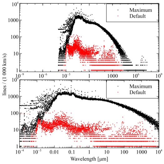
Fig. 2 This shows the number of lines that fall into 1000 km/s velocity bins, across the spectrum. The red points for default setup and the black points give the number of lines the are predicted when the databases are made as large as possible. The upper panel shows the full spectral range considered by the code, while the lower panel shows the peak of the line density. The color figure can be viewed online.
We will give example input scripts across this document to show how various Figures were produced. The large-database calculation in Figure 2 was created with the following input deck:
table AGN
ionization parameter -2
stop zone 1
constant temperature 1e4 K hden 0
database H2
database H-like levels resolved 5
database He-like levels resolved 5
database H-like levels collapsed 200
database He-like levels collapsed 200
database CHIANTI levels máximum
database stout levels máximum
database LAMDA levels maximum
save continuum units microns "mesh.con"
All commands are fully documented in “Hazy 1”, CLOUDY’s documentation, which is part of the download. Most commands are unchanged from C13. The spectral energy distribution (SED) is our generic Active Galactic Nucleus (AGN) continuum, with an ionization parameter of U = 10−2. The geometry is a single zone with a hydrogen density of 1 cm−3 and a gas kinetic temperature set to 104 K. These have to be specified to get the code to run and were chosen to do the simplest and fastest calculation. As described here, the database commands are new in C17 and control the behavior of the databases.
The number of lines per spectral bin is one of the items in the file produced by the save continuum command. The width of each continuum bin, or, equivalently, the spectral resolution, can be adjusted in two ways. The default continuum mesh can be changed by a uniform scale factor with the set continuum resolution ... command. This method is used in several simulations presented below to increase the spectral resolution to highlight particular issues in the spectrum. Alternatively, the initialization file continuum mesh.ini in the data directory can be changed to alter the default continuum mesh. This second method was used to make the C13 and C17 continuum meshes the same, to allow the comparison in Figure 1.
Figure 2 shows that it is possible to predict a very large number of lines, but this comes at great cost. The default C17 calculation took 4.3 s on an Intel Core I7 processor while the calculation using the large databases took 1822 s, roughly half an hour. It would not now be feasible to use the full databases in a realistic calculation in which the temperatura solver is used and the cloud has a significant column density so that optical depths are important.
2.6.1. database print
The command database print generates a report listing all species. The following would generate a report for CLOUDY in its default setup:
This command was used to generate Tables 2 and 3 giving the default setup for the one-and two-electron iso-sequences. A small portion of the report for the Stout, CHIANTI, and LAMDA databases follows:
Using LAMDA model SO with 70 levels of 91 available.
Using LAMDA model SiC2 with 40 levels of 40 available.
Using LAMDA model CS with 31 levels of 31 available.
Using LAMDA model C2H with 70 levels of 102 available.
Using LAMDA model OH+ with 49 levels of 49 available.
Using STOUT spectrum Al 1 (species: Al) with 15 levels of 187 available.
Using STOUT spectrum Al 3 (species: Al+2) with 15 levels of 83 available.
Using STOUT spectrum Al 4 (species: Al+3) with 15 levels of 115 available.
Using STOUT spectrum Zn 2 (species: Zn+) with 15 levels of 27 available.
Using STOUT spectrum Zn 4 (species: Zn+3) with 2 levels of 2 available.
Using CHIANTI spectrum Al 2 (species: Al+) with 15 experimental energy levels of 20 available.
Using CHIANTI spectrum Al 5 (species: Al+4) with 3 experimental energy levels of 3 available.
Using CHIANTI spectrum Al 7 (species: Al+6) with 15 experimental energy levels of 15 available.
Using CHIANTI spectrum Al 8 (species: Al+7) with 15 experimental energy levels of 20 available.
Using CHIANTI spectrum Al 9 (species: Al+8) with 15 experimental energy levels of 54 available.
Table 1 Save species label example
| Species label | Database |
| H | H-like |
| H+ | |
| H- | |
| He | He-like |
| He+ | H-like |
| He+2 | |
| HeH+ | |
| C | Stout |
| C+ | Stout |
| C+2 | Stout |
| C+3 | CHIANTI |
| C+4 | He-like |
| C+5 | H-like |
| C+6 | |
| C2+ | |
| C2H | LAMDA |
| NH3 | LAMDA |
| CN | LAMDA |
| CN+ | |
| HCN | LAMDA |
Table 2 Default number of levels for the h-like iso-electronic sequence
| Element | n(res) | nls(res) | n(coll) |
| H | 10 | 55 | 15 |
| He | 10 | 55 | 15 |
| Li | 5 | 15 | 2 |
| Be | 5 | 15 | 2 |
| B | 5 | 15 | 2 |
| C | 5 | 15 | 5 |
| N | 5 | 15 | 5 |
| O | 5 | 15 | 5 |
| F | 5 | 15 | 2 |
| Ne | 5 | 15 | 5 |
| Na | 5 | 15 | 2 |
| Mg | 5 | 15 | 5 |
| Al | 5 | 15 | 2 |
| Si | 5 | 15 | 5 |
| P | 5 | 15 | 2 |
| S | 5 | 15 | 5 |
| Cl | 5 | 15 | 2 |
| Ar | 5 | 15 | 2 |
| K | 5 | 15 | 2 |
| Ca | 5 | 15 | 2 |
| Sc | 5 | 15 | 2 |
| Ti | 5 | 15 | 2 |
| V | 5 | 15 | 2 |
| Cr | 5 | 15 | 2 |
| Mn | 5 | 15 | 2 |
| Fe | 5 | 15 | 5 |
| Co | 5 | 15 | 2 |
| Ni | 5 | 15 | 2 |
| Cu | 5 | 15 | 2 |
| Zn | 5 | 15 | 5 |
Table 3 Default number of levels for he-like iso-electronic sequence
| Element | n(res) | nls(res) | n(coll) |
| He | 6 | 43 | 20 |
| Li | 3 | 13 | 2 |
| Be | 3 | 13 | 2 |
| B | 3 | 13 | 2 |
| C | 5 | 31 | 5 |
| N | 5 | 31 | 5 |
| O | 5 | 31 | 5 |
| F | 3 | 13 | 2 |
| Ne | 5 | 31 | 5 |
| Na | 3 | 13 | 2 |
| Mg | 5 | 31 | 5 |
| Al | 3 | 13 | 2 |
| Si | 5 | 31 | 5 |
| P | 3 | 13 | 2 |
| S | 5 | 31 | 5 |
| Cl | 3 | 13 | 2 |
| Ar | 3 | 13 | 2 |
| K | 3 | 13 | 2 |
| Ca | 3 | 13 | 2 |
| Sc | 3 | 13 | 2 |
| Ti | 3 | 13 | 2 |
| V | 3 | 13 | 2 |
| Cr | 3 | 13 | 2 |
| Mn | 3 | 13 | 2 |
| Fe | 5 | 31 | 5 |
| Co | 3 | 13 | 2 |
| Ni | 3 | 13 | 2 |
| Cu | 3 | 13 | 2 |
| Zn | 5 | 31 | 5 |
Each line of output gives the database name, the spectroscopic designation, the species designation, the number of levels used, and the total number available. With CHIANTI there is the further option to use all levels, or only those with experimental (measured) energies.
2.6.2. save species labels all
The save species labels all command will produce a file containing the full list of species labels. One can generate this list by running the following input deck:
Table 1 shows a small part of the resulting output. There are several important points in this Table. First, several species do not list a database. The cases of “H+”, “He+2”, and “C+6” are bare nuclei and have no electronic levels, while the negative hydrogen ion“H-” and the molecules “HeH+”, “C2+” and “CN+” do have internal levels in nature, but we currently do not have models of these systems. The remainder are treated with one of the databases described above. Although many of these species have no internal structure, other species properties, especially the column density, are computed and reported.
Note a likely source of confusion. As described above, “C+2” is doubly ionized carbon, while “C2+” is an ion of molecular carbon.
2.6.3 print citation
The print citation command reports the ADS links to papers defining the databases we use. We encourage users to cite the original source of any data that played an important role in an investigation. This will support and encourage atomic, molecular, and chemical physicists to continue their valuable work.
2.6.4. save species Commands
It is easy to report internal properties of a species, such as the column density or population of a particular level. The following is an example of a save species command used to report the column densities of several species and the visual extinction:
The total column density of electrons, H2, H0, and H+ would be reported, along with the population in the J = 1 level of CO, and the first five levels of C0. Note that the level index within the “[xx:yy]” counts from a lowest level of 1.
2.6.5. Save line labels
The save line labels command creates a file listing all spectral-line labels and wavelengths in the same format as they appear in the main output’s emission-line list. This is a useful way to obtain a list of lines to use when looking for a specific line. The file is tab-delimited, with the first column giving the line’s index within the large stack of spectral lines, the second giving the character string that identifies the line in the output, and the third giving the line’s wavelength in any of several units. Each entry ends with a description of the spectral line. Lines derived from databases (CHIANTI, Stout, LAMDA) are followed by a comment that contains the database of origin and the indices of the energy levels, as listed in the original data.
An example of some of its output follows:
4 Inci 0 total luminosity in incident continuum
5 TotH 0 total heating, all forms, information since individuals added later
6 TotC 0 total cooling, all forms, information since individuals added later
1259 H 1 911.759A radiative recombination continuum
1260 H 1 3646.00A radiative recombination continuum
1261 H 1 3646.00A radiative recombination continuum
1262 H 1 8203.58A radiative recombination continuum
3552 H 1 1215.68A H-like, 1 3, 1^2S - 2^2P
3557 H 1 1025.73A H-like, 1 5, 1^2S - 3^2P
3562 H 1 972.543A H-like, 1 8, 1^2S - 4^2P
5328 Ca B 1640.00A case a or case b from Hummer & Storey tables
5329 Ca B 1215.23A case a or case b from Hummer & Storey tables
73487 CO 2600.05m LAMDA, 1 2
73492 CO 1300.05m LAMDA, 2 3
73497 CO 866.727m LAMDA, 3 4
85082 C 3 1908.73A Stout, 1 3
85087 C 3 1906.68A Stout, 1 4
85092 C 3 977.020A Stout, 1 5
180217 Al 8 5.82933m CHIANTI, 1 2
180222 Al 8 2139.33A CHIANTI, 1 4
180227 Al 8 381.132A CHIANTI, 1 8
312763 H2 1.13242m diatoms lines
312768 H2 1.26316m diatoms lines
312854 Blnd 2798.00A Blend: "Mg 2 2795.53A"+"Mg 2 2802.71A"
312855 Blnd 615.000A Blend: "Mg10 609.794A"+"Mg10 624.943A"
3. THE IONIZATION EQUILIBRIUM
Our goal is to compute the ionization for a very wide range of densities and temperatures, as shown in Figures 17 and 18 of C13, for the first thirty elements and all of their ions.5 This development is complete for the H- and He-like iso-electronic sequences, but is still in progress for many-electron systems. This is challenging because of limitations in the available atomic data, computer hardware, and human effort. We currently use a hybrid scheme, outlined below, which is motivated by the astrophysical problems we wish to solve. Figure 3 shows energy levels for five typical species, to serve as an example of some of the issues involved in the following discussion.

Fig. 3 Experimental energy levels (Kramida et al. 2014) for some species present in an ionized gas. The energies are given relative to the ionization potential (IP). Of these ions, only O III and Mg II have data for autoionizing levels, shown as the levels above the ionization limit indicated by the red hashed box. The autoionizing levels of Mg II are not visible since they are far above the ionization limit. The vertical bar in the middle, corresponding to E/IP = 0.05, is a typical gas kinetic energy in a photoionized plasma and is shown to indicate which levels are energetically accessible from the ground state. The color figure can be viewed online.

Fig. 4 Ratios of He I lines using the different datasets with respect to PS-M, see text for details. Figure from (Guzmán et al. 2017b). The color figure can be viewed online.

Fig. 5 This shows ratios of our predicted H i emission to the Storey & Hummer (1995) Case B tables. Calculations are for Te = 104 K and the indicated densities. The upper panel, our test case limit caseb h den4 temp4.in., shows that we reproduce their results to high accuracy when a large model is used. The default model, chosen as a compromise between speed and accuracy, is shown in the lower two panels. The default model is designed to give higher accuracy for the brighter optical and near-IR lines, plotted as the larger filled circles. Note that each panel has a different vertical scale. The color figure can be viewed online.

Fig. 6 This shows ratios of our predicted H i emission to the Storey & Hummer (1995) Case B tables for our default Hi model. Calculations are for the full temperature and density range they provide. Major contours are at I/ICaseB = 0.5,1, and 1.5 while minor contours, shown as the dotted lines, are at 10% incremental values. The differences at the higher densities are due to the use of more recent collision rates in our calculations.

Fig. 7 This compares emission around the Balmer jump for the Case B models used in Figure 5. The continuum resolution is increased by a factor of ten above our default with the command set continuum resolution 0.1. The upper and lower panels compare the emission predicted by the large and default models. The large model reproduces the correct smooth merging of the lines and continuum, while the “gap” introduced by the finite size of our default H0 model is obvious in the lower panel. The color figure can be viewed online.

Fig. 8 The transmitted continuum in the region around the Lyman jump is for our default model, which includes “extra” Lyman lines extending to n = 100. The highn Lyman lines merge into the Lyman continuum. The vertical line indicates the wavelength of the Lyman jump. The continuum resolution has been increased by a factor of ten above our default.

Fig. 9 The emitted spectrum of an optically thin photoionized cloud with solar abundances. The upper panel uses our default models while the lower panel is an enlarged model. The continuum resolution is increased by a factor of ten above our default.

Fig. 10 Ionization of hydrogen as a function of density. The low-density coronal approximation limit occurs on the left, while the thermodynamic statistical equilibrium limit applies at high densities. The solid black line is the full numerical CRM solution, the red dashed line is the ionization predicted by the two-level approximation, and the dasheddotted line is the prediction of the Saha-Boltzmann equation. The color figure can be viewed online.

Fig. 11 Density ratio of fully-ionized to single-electron species as a function of electron density. The plot is for different elements with nuclear charge indicated. The effects of increasing charge on the range of validity of the coronal and LTE limits are dramatic.

Fig. 12 As in Figure 11, but for the photoionization case. The CRM peak, prominent in Figure 11 and produced by collisional ionization from highly-excited levels, is not present because the Rydberg levels that enhance the ionization have a smaller population in photoionization equilibrium.
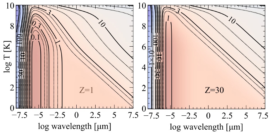
Fig 13 Values of the gIII Gaunt factor over the full wavelength, temperature, and nuclear charge range CLOUDY considers.

Fig. 14 This shows two of the quantities that enter into the S59 calculation of gII . The vertical dotted line marks the point where SD93 claim that Seaton’s theory is discontinuous. The dashed-dotted lines give the quantities plotted in the lower panel of Figure 1 of SD93. The dashed curves give SD93’s “corrected Seaton” theory. The heavy solid lines give our recalculation of the terms S and σ using Seaton’s original expressions and tables.

Fig. 15 Hydrogenic recombination rate coefficients are shown vs. reduced temperature, T/Z2, for the ground state, n = 1. The vertical dotted line marks the SD93 discontinuity, where the theory changes from the numerical to analytical forms. The dashdotted line gives SD93’s evaluation of the Seaton rate, taken from the upper panel of their Figure 1. The dashed line is SD93’s “corrected Seaton” theory. The heavy solid line gives our recalculation of the rates using Seaton’s original expressions and tables. All the rates are multiplied by the reduced temperature.

Fig. 16 Comparison of various hydrogenic total Case B recombination rate coefficients. Our reevaluation of Seaton’s theory is shown as the heavy solid line drawn over the temperature range where he said it was applicable. The dot-dashed line gives the rate used in Mappings I, equation (7) of SD93. The SD93 “corrected Seaton” rate is shown as the long dashed line. The short dashed line gives the F92 rates derived by direct numerical integration of the Milne equation over hydrogenic photoionization cross sections. The F92 curve lies behind the Seaton curve for T < 106 K, the temperature range he indicated the theory was accurate. All rate terms are multiplied by a factor of T/Z2.

Fig. 17 This compares the effects of our different PAH abundance laws in the Leiden F1 PDR model. The upper panel shows the electron density for the three cases, see text for details. The constant and "H,H2" cases overlap because there is very little H+ in this model. The lower panel shows fractional abundances, for the "H" case, for some of the important species in a PDR.
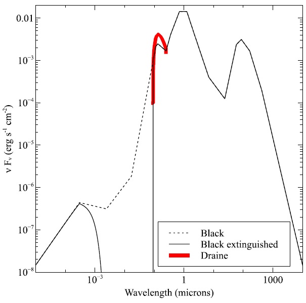
Fig. 18 The SED produced by the table ISM command is the lighter line. The infrared cirrus is the peak at λ ∼ 100 µm and starlight dominates at shorter wave- lengths. The points just shortward of the Lyman limit (0.0912 µm) are interpolated-actually it is thought that interstellar extinction removes most of this continuum. The dashed line shows the interpolated SED and the solid line shows the effects of absorption introduced by adding the extinguish command. The heavy red line is SED produced the table Draine continuum and used in many PDR calculations. The color figure can be viewed online.
There are two simple limits for the solution of the ionization equilibrium. At the low densities found in the interstellar medium (ISM), most ions are in the ground state and the ionization rate per unit volume is proportional to the atom density multiplied either by the electron density, in the case of collisional ionization, or the ionizing photon flux, in the case of photoionization. The recombination rate per unit volume is proportional to the product of the ion and electron density. The density dependence drops out for the case of collisional ionization (see Equation 4 below). In contrast, at very high densities, such as the lower regions of a stellar atmosphere, the ionization is given by the Saha-Boltzmann equation and is inversely proportional to the electron density (Equation 5 below). CLOUDY spans both regions so neither approximation can be made and a full solution of the NLTE equations should be performed to obtain the ionization balance and level populations.
In a collisional-radiative model (CRM), the name given to the full NLTE treatment in plasma physics, the level populations are determined self-consistently with the ionization. That is, the populations in bound levels and the continuum above them in Figure 3 are solved as a coupled system of equations. We use this approach for the H-like and He-like isosequences, as described in C13 and the following sections, and shown in Figures 17 and 18 of C13. A modified two-level approximation, described below, is used for other species. This hybrid approach is motivated by the physics of the systems shown in Figure 3.
3.1. The H- and He-like Iso-electronic Sequences
Energy levels for H0 are shown in Figure 3 on the left. This structure is valid for all ions of the H-like isoelectronic sequence. For H0, the first excited n = 2 level occurs at an energy E ≈ (1 − 1/n2) ≈ 0.75 of the ionization limit. This lowest excited level is much closer to the continuum above it than to the ground state below it. At the low kinetic temperatures found in photoionization equilibrium there should be little collisional coupling between excited and ground states because of this large energy separation, although very highly excited levels are strongly coupled to the continuum above. As a result, the very highly excited “Rydberg” levels are populated following recombination from the ion above it, rather than collisional excitation from the ground state, in photoionization equilibrium. Most optical and infrared emission is produced following recombination in this case. The energies of the nshells are also roughly valid for the He-like sequence. These two-electron systems behave in a similar manner; optical and IR lines form by recombination.
We treat these two iso-electronic systems with a full CRM because of the strong coupling of excited level populations to the continuum (C13). A large coupled system of equations is solved to determine both the level populations and the ionization, so the two are entirely self-consistent. Predictions over a wide range of density and temperature are shown in Figures 17 and 18 of C13. We developed a unified model for both the H-like and He-like isoelectronic sequences that extends from H to Zn, as described by Bauman et al. (2005); Porter et al. (2007); Porter & Ferland (2007); Porter et al. (2012) and Luridiana et al. (2009), As shown in C13, and previously by Ferland & Rees (1988), our model of the ionization and chemistry of hydrogen does go to the correct limits at high (LTE) and low (ISM) densities, and to the strict thermodynamic equilibrium (STE) limit when exposed to a true blackbody. This is only possible when the ionization and level populations are self-consistently determined by solving the full collisional-radiative problem.
3.1.1. Recent Developments
The Hand He-like isoelectronic-sequences, coupled with the cosmic abundances of the elements, cause their spectra to fall into two very different regimes. For brevity, we refer to these as isosequences in the following. Hydrogen and helium have low nuclear charge Z and so have low ionization potentials, IP ∼ Z2. As a result, H i, He i, and He ii emission is produced in gas with nebular temperatures, ≈ 104 K, and occurs mainly in the optical and infrared. A goal of the current development is the prediction of highly accurate line emissivities as a step towards measuring the primordial helium abundance (Porter et al. 2007).
The next most abundant elements, starting with carbon (Z = 6), have high ionization potentials, IP ≥ 62 Ryd, so are produced in very hot gas, T ≥ 106 K, and emit X-rays (Porter & Ferland 2007; Porter et al. 2006). Heavy elements of these iso-sequences fall into very different spectral regimes than hydrogen and helium, probe gas with very different physical conditions, and so are found in distinctly different environments.
The high precision needed for primordial helium measurements means that the atomic data must be quite accurate. We are revisiting this problem. The original papers on H i and He i emission (Brocklehurst 1971, 1972; Benjamin et al. 1999; Hummer & Storey 1987) all used the Pengelly & Seaton (1964) theory of lchanging collisions. Vrinceanu & Flannery (2001b,a) and Vrinceanu et al. (2012) present an improved theory for these collisions, which predict rate coefficients that are ≈6 times smaller. We have used these newer rates in most of our published work (Bauman et al. 2005; Porter et al. 2007; Porter & Ferland 2007; Porter et al. 2012; Luridiana et al. 2009), and in C13.
There are good reasons, outlined in Guzmán et al. (2016), to prefer the Pengelly & Seaton (1964) theory. Guzmán et al. (2017b) extend this treatment to He-like systems, in which the low-l S, P, and D states are not energy-degenerate, so an extra cut-off energy term is applied to the probability integral as in Pengelly & Seaton (1964). Guzmán et al. (2017b) also improve the Pengelly & Seaton (1964) approximations to deal with low densities and high temperatures, where the original formulae could produce negative values. They call this the modified Pengelly & Seaton (1964, PS-M) approach. Williams et al. (2017) extend the semi-classical theory of Vrinceanu & Flannery (2001b) to provide thermodynamically consistent l-changing rates, which are found to agree quite closely with the results of the other approaches. These differences affect the predictions. In Figure 4, the line emissivities from the different approaches are divided by the emissivities obtained using PS-M Here, a single layer of gas has been considered and emissivities from recombination lines calculated. A cosmic helium abundance, He/H =0.1, was assumed. The cloud is radiated by a monochromatic radiation field using CLOUDY’s laser command. It was centered at 2 Ryd, with an ionization parameter of U = 0.1 (Osterbrock & Ferland 2006). The state of the emitting gas in these conditions resembles that in Hii regions, observationally relevant for the determination of He abundances (Izotov et al. 2014). The monochromatic radiation field was used to prevent internal excitations that would be produced by a broadband incident radiation field. A constant gas kinetic temperature of 1×10⁴ K is assumed. We assume ‘Case B’ (Baker & Menzel 1938), where Lyman lines with upper shell n > 2 are assumed to scatter often enough to be degraded into Balmer lines and Lyα. The hydrogen density is varied over a wide range and the electron density is calculated self-consistently. The latter is approximately 10% greater than the hydrogen density, since He is singly ionized. The atomic data used for He and H emission, except for l-changing collisions, are the ‘standard’ set of data that have been described in previous work (Porter et al. 2005).
In Figure 4, the most accurate quantum mechanical treatment, VOS12-QM (Vrinceanu & Flannery 2001a b, a; Vrinceanu et al. 2012), agrees closely with PS-M. The semiclassical treatments, VOS12-SC (Vrinceanu & Flannery 2001b,a), and the further simplified approach, VOS12-SSC (Vrinceanu et al. 2012), produce differences of up to 10% in the predicted line intensities. The input to generate Figure 4 for the quantum mechanical case can be as follows6:
laser 2
ionization parameter -1
hden 4
element helium abundance -1
init file "hheonly.ini" stop zone 1
set dr 0
database he-like resolved levels 30
database he-like collapsed levels 170
database he-like collisions l-mixing S62 \
no degeneracy thermal VOS12 quantal
constant temperature 4
case b no photoionzation no Pdest
no scattering escape
no induced processes
iterate
normalise to "He 1" 4471.49A
monitor line luminosity "He 1" 7281.35A \
-18.8686
In this input, the no photoionization option is added to case b to suppress photoionization from excited levels. Then, the pumping of the levels by the resulting photon field is removed by turning off the destruction of Lyman lines with the no Pdest option. The density is set to 104 cm−3 using the hden 4 command, and the temperature is kept constant with constant temperature 4. The commands:
stop zone 1
set dr 0
define a layer of gas of 1 cm thickness. The commands:
no scattering escape no induced processes
prevent losses due to scattering, so that all Lyman lines are degraded into Balmer lines. The monitor line luminosity ... command compares the computed luminosities (erg s−1) of selected He i lines against the reference values given by the PS method. Luminosities can be directly translated into emissivities as the thickness of the gas is 1 cm.
Figure 4 has been computed extending to the n = 200 shell using the database he-like resolved/collapsed levels commands described in § 3.1.2. Most of the higher n-shells are collapsed (C13, Figure 1) assuming a statistical population for the l-subshells, while the low-n levels are resolved. The number of resolved levels needed is determined by the critical density for l-mixing, where collisional transition rates exceed radiative decay rates, as shown in Figure 4 of Pengelly & Seaton (1964). The number of resolved n-shells used to predict the lines in Figure 4 has been varied from n = 60 at the lowest density to n = 20 at the highest density.
Commands are provided to select the preferred l-changing theory in the input file for CLOUDY. The command to use PS-M is:
The keyword S62 in this command tells CLOUDY to use the Seaton (1962) electron impact cross sections for the l-changing collisions of the highly nondegenerate l < 3 subshells (see Guzmán et al. 2017b). The keyword no degeneracy uses an energy criterion (Pengelly & Seaton 1964) to account for the non-degeneracy of the l-subshells of He i Rydberg levels (see above). Calculations using the original formulas provided by Pengelly & Seaton (1964) can be used by adding the keyword Classic.
VOS12-QM rate coefficients can be used with the command:
where the keyword thermal tells CLOUDY to perform a Maxwell average for the cross sections. By default, the effective coefficients will not be Maxwell averaged, and energies of the collision particles will be taken to be kT . The evaluation at a single energy kT is significantly faster.
The VOS12-QM theory needs a larger number of operations than the analytic PS-M approach. It also needs a numerical integration of the collision probability to obtain the cross sections. These may be integrated once more to obtain the Maxwell averaged coefficients, making this method computationally slow. Simulations using VOS12-QM calculations are ≈ 60 times slower than those using PS-M. The computational cost of VOS12-QM calculations makes PS-M method the preferred one. The VOS12-QM method is recommended when very high-precision results are required.
Finally VOS12-SC and VOS12-SSC can be obtained using the commands:
database he-like collisions l-mixing S62 \ thermal Vrinceanu
database he-like collisions l-mixing S62 \ VOS12 semiclassical
respectively. While VOS12-SSC cross-sections can be obtained with an analytical formula, VOS12-SC need a double integration making them as computationally slow as VOS12-QM.
It is not now possible to experimentally determine which of the theories mentioned above is more correct, although we prefer the PS-M approach. Guzmán et al. (2017a) outline an astronomical observation that, while difficult, could conclusively determine which l-changing theory holds.
3.1.2. Adjusting the Size of the Model
Our models of the Hand Helike iso-sequences have a mixture of resolved and collapsed levels, as shown in Figure 1 of C13. Resolved levels are relatively expensive to compute due to the need to evaluate the l-changing collision rates described above. Collapsed levels assume that the l-levels are populated according to their statistical weight within the n shell, so this expense is avoided.
The number of resolved and collapsed levels are controlled by a family of commands similar to
database H-like hydrogen levels resolved 10
database H-like hydrogen levels collapsed 30
database H-like helium levels resolved 10
database H-like helium levels collapsed 30
database He-like helium levels resolved 10
database He-like helium levels collapsed 30
This example resolves n ≤ 10 for H i, He i, and He ii and adds 30 collapsed levels to make each atom extend through n = 40. These commands work for
H-like and He-like ions of all elements up through zinc (Z=30).
The command:
generates a report summarizing all databases in use during the current calculation. This includes the number of resolved and collapsed levels for the isosequences. By default we resolve n ≤ 10 with an additional 15 collapsed levels for H i and He ii, and n ≤ 6 as resolved with an additional 20 collapsed levels for He i.
In C13 and earlier versions the collapsed levels were intended to “top off” the model and their treatment did not have spectroscopic accuracy. Bauman et al. (2005) discuss top off, the need to use a finite number of levels to approximate an infinite-level system, and its effects on predictions. We did not report lines from collapsed levels. A great deal of effort has gone into improving the physics of these levels. Their emission is now highly accurate if the implicit assumption that the l levels within the n shell are populated according to their statistical weight is valid. The densities required for this “well l-mixed” assumption can be derived from Figure 4 of Pengelly & Seaton (1964). We now report emission from collapsed levels up to n < nhighest − 4. This limit was chosen to avoid the “edge” effects discussed in the next subsection.
3.1.3. Comparisons in the Case B Limit
It is possible to judge the accuracy of the predicted lines by comparing with the textbook “Case B” spectrum (Baker & Menzel 1938). Case B is a well defined limit that is a fair approximation to nebulae (AGN3 § 4.2) and can serve as an important benchmark. Hummer & Storey (1987) and Storey & Hummer (1995) compute Case B emission and the second paper includes a series of machine-readable tables. We interpolate on these tables to include Case B predictions for H-like ions in the CLOUDY output. This makes comparison of our predictions with Case B simple.
While Case B is an idealized limit, it gives a fairly good representation of emission for low to moderate density photoionized nebulae (AGN3). The assumptions break down if Balmer or higher lines become optically thick, when collisional excitation from the ground state becomes important, or if Lyman lines can escape. Optical depth effects become important in high radiation-density environments such as the inner regions of active galactic nuclei. Collisional contributions become important when suprathermal electrons are present as in X-ray ionized neutral gas (Spitzer & Tomasko 1968), or for hot regions such as very low metallicity nebulae. The Lyman lines may not be optically thick in low column density clouds. These processes are treated self-consistently in any complete CLOUDY calculation.
Larger models, with more levels, make the spectrum more accurate, at the cost of longer execution times and higher memory requirements. The default H i model is a compromise between performance and accuracy.
Figure 5 compares our predictions with Storey & Hummer (1995) for a typical “nebular” temperature, Te = 104 K, and two densities, n(H) = 104 cm−3 and 107 cm−3. The lower two panels show predictions of our default model at the two densities while the upper panel shows predictions at the lower density with a greatly increased number of resolved and collapsed levels.
In a normal calculation, CLOUDY determines the line optical depths self-consistently, assuming the computed column densities, level populations, and line broadening. A Case B command exists to create these conditions and to make these comparisons possible while computing a single “zone”, a thin layer of gas. The command sets the Lyman line optical depth to a large number and suppresses collisional excitation out of n = 2, to be consistent with the Storey & Hummer (1995) implementation of Case B. This command was included in the input script used to to create Figure 5. In previous versions of CLOUDY we also recommended using the Case B command in certain simple PDR (photodissociation region, or photon-dominated region) calculations to block Lyman line fluorescence. As described in § 5.4 below, we now recommend using a different command in the PDR case, reserving the Case B command for this purpose only.
The large model reproduces the Storey & Hummer (1995) results to high precision. There are differences at the ∼ 2% level, which we believe to be caused by recent improvements in the collision and recombination data. This will be the subject of a future paper (Guzmán et al. in preparation).
The middle and lower panels show the results of applying our default H i model (n ≤ 10 resolved with an additional 15 collapsed) to the same density, and to a higher density case. The default model was chosen to reproduce the intensities of the brighter H i lines to good precision. The large red filled circles in the middle panel indicate lines with intensities greater than 5% that of Hβ. These have deviations of <∼ 10%.
The eye picks up a trend for the error ratio to move away from unity along a spectroscopic (that is, Balmer, Paschen, etc) series, as the upper level n increases. This is produced by two effects. The first is an “edge” effect as the upper level approaches the upper limit of the model. (We do not report lines arising from n ≥ nhighest − 4 for this reason.) The level populations for the very highest levels are inaccurate because of their proximity to the large “gap” that exists between the highest level and the continuum above. The errors at lower n are due to the fact that the lower collapsed levels, 10 < n ≤ 15, are not actually l-mixed at the lower density of 104 cm−3. The density of 107 cm−3 is high enough to l-mix n = 11 so this model is better behaved. These tests show that the implementation gives reliable results when the number of levels is made large enough.
The default model was designed to reproduce the intensities of the brighter H i lines while being computationally expeditious. As a test we computed the intensities of four of the most commonly observed H i lines over the density and temperature given in the Storey & Hummer (1995) tables including the Case B command. The ratio of our predictions to their Case B values is given in Figure 6. The largest differences are at the higher densities where Case B would not be expected to apply. These differences are due to recent improvements in the H0 collision rates. At the lower densities where Case B might apply the agreement is good; the default model is generally within 10% of Storey & Hummer (1995).
This calculation used our grid command to compute the required range of density and temperature and the save linelist ratio command to save predictions into a file. The input script is
set save prefix "nt"
case B
hden 4 vary
grid 2 14 .5 log
constant temperature 4 vary
grid 2.7 4.4 0.05 log
#
stop zone 1
set dr 0
laser 2
ionization parameter 0
init "honly.ini"
save grid ".grd"
save linelist ratio ".rat" "nt.lines" last no hash
The save linelist ratio command reads the list of lines in the file nt.lines and saves them into the file nt.rat. The list of lines in nt.lines are ordered pairs and the ratio of intensities of the first to second is reported. (The “#” lines are comments added to aid the user and are ignored.) The predictions in the nt.rat file were combined with the grid model parameters saved in the file nt.grd to créate the plot. The nt.lines file contained the following set of line ratios:
| H | 1 | 4340.49A |
| Ca | B | 4340.49A |
| # | ||
| H | 1 | 4861.36A |
| Ca | B | 4861.36A |
| # | ||
| H | 1 | 6562.85A |
| Ca | B | 6562.85A |
| # | ||
| H | 1 | 1.87511m |
| Ca | B | 1.87511m |
| # | ||
| H | 1 | 2.16553m |
| Ca | B | 2.16553m |
Similar tests can be made for other lines of interest.
The number of resolved levels must be increased when higher precision is needed at low densities (Figure 6) or for faint IR / FIR lines (Figure 5). Figure 4 of Pengelly & Seaton (1964) can be used as a guide in deciding how many resolved levels are needed. Their vertical axis is, in effect, the negative log of the hydrogen density. The lines indicate the critical density, defined in eqn 3.30 of AGN3, where l-changing rates are equal to the radiative decay rate. The l levels within the indicated n will be well mixed when the density is significantly higher than this critical density. For instance, at a density of 104 cm−3, the figure shows that the n = 15 shell is at its critical density. Our default model uses collapsed levels for 11 ≤ n ≤ 15, causing the residuals in the center panel of Figure 5. Our lowest collapsed level, n = 11, has a critical density of ∼ 105.5 cm−3. This is why the model is so much more accurate, but still not excellent, at the higher density in the lower panel, 107 cm−3.
The user could adjust the model to suit requirements at a particular density using Case B predictions as a guide. We recommend creating a one-zone Case B simulation with a density and temperature set to the conditions under study. Then, adjust the size of the model to achieve the desired accuracy by comparing the lines of interest with the Storey & Hummer (1995) Case B predictions that are included in the output.
Making the model large does come at some cost. Tests show that the test suite example pn paris, one of the original Meudon meeting test cases (Péquignot 1986), takes ≈ 27s using the default H0 model on a modern Xeon, while the large model in Figure 5 takes 44m 25s.
3.1.4. Convergence of Lines onto Radiative Recombination Continua
As mentioned above, the finite size of the H0 model is one source of deviations from Case B line predictions in Figure 5. Any finite model will have a “gap” between the highest level and the continuum above. This gap is also present in the predicted spectrum, as shown in Figure 7. This shows the converging high-n Balmer lines and the Balmer jump corresponding to radiative recombination captures to n = 2. The upper panel shows the large model used in Figure 5 while the lower is the default model. There is no “gap” in the large model, or in nature, but rather the Balmer lines merge onto the Balmer jump. This is correct and due to the fact that the oscillator strength is continuous between high-n Balmer lines and the Balmer continuum (Hummer & Storey 1998). The “gap” in the default model is obvious at this high resolution. We note that Schirmer (2016) presents similar figures.
Lyman absorption lines do not suffer from the complexities of H i emission lines since absorption lines depend on the population of the lower level, the ground state in this case. It is then simple to include an arbitrary number of “extra” Lyman lines, lying above the explicit model, so that “gaps” do not appear. An example is shown in Figure 8, a high-resolution blow-up of the spectral region around the Lyman jump. The calculation used our default H0 model. It is a solar abundance cloud illuminated by our generic AGN SED, with an ionization parameter of log U = −2, a column density of N (H0) = 1018 cm−2 , and does not assume Case B. The smooth blending into the Lyman jump is the correct behavior. All iso-sequence models are topped off with these extra Lyman lines.
3.1.5. The Hand He-like Ions in the X-ray
The entire H-like and He-like series of ions between HI and Zn XXX are treated with a common code base and have the same commands to change their behavior. Porter & Ferland (2007) discuss the treatment with an emphasis on the changes in the He-like X-ray emission due to UV photoexcitation of the metastable 2 3S level. Mehdipour et al. (2016) compare the X-ray spectral predictions of C13 with the Kaastra (SPEX) and Kallman (XSTAR) codes and find reasonable agreement.
The default number of levels for the H-like and He-like iso-electronic sequences are summarized in Tables 2 and 3. The issues discussed above carry over into the X-ray region. Figure 9 shows a small portion of the emission spectrum of a solar abundance cloud photoionized by our generic AGN continuum. The ionization parameter was adjusted to log U = 100.75 to insure that C, N, and O were present as H-like and He-like ions.
The “gap” between the recombination edges and the converging Lyman lines is evident in the upper panel. It is larger than in the H i case because we use relatively few levels for these high-ionization species (see Tables 2 and 3). The number of collapsed levels was increased to predict the spectrum in the lower panel. This larger model was computed with the input stream
set save prefix "large"
set continuum resolution 0.1
c only include H, C, N, and O, with an increased
c number of collapsed levels
database H-like levels collapsed 20
database He-like levels collapsed 20
table agn
ionization parameter 0.75
hden 0
stop zone 1
set dr 0
iterate
print last iteration
save emitted continuum ".con" last units Angstroms
The extra levels produce enough lines to fill in the “gap” at this resolution. Regions of significantly increased emission produced by the additional levels are also evident in the larger model.
3.2.1. The Two-level Approximation
Textbooks on the interstellar medium (ISM), e.g. Spitzer (1978), Tielens (2005), Osterbrock & Ferland (2006), and Draine (2011), write the ionization balance of an ion as the equivalent two-level system:
where n(i + 1) and n(i) are the densities of two adjacent ionization stages, α(i + 1) is the total recombination rate coefficient of the ion (cm3 s−1) and Γ(i) is the ionization rate (s−1). In photoionization equilibrium
where φν is the flux of ionizing photons [photons s−1 cm−2 Hz−1], σν is the photoionization cross section [cm−2] and the integral is over ionizing energies. On the other hand, in collisional ionization equilibrium
where q(i) is the collisional ionization rate coefficient.
In its simplest form, the two-level approximation assumes that recombinations to all excited states will eventually decay to the ground state, and that all ionizations occur out of the ground state. Only the ionization rate from the ground state and the sum of recombination coefficients to all excited states need be considered, a great savings in data needs.
This two-level approach extends over to the chemistry. Most codes use databases similar to the UMIST Database for Astrochemistry (McElroy et al. 2013). Reactions between complex molecules are treated as a single channel without detailed treatment of internal structure. In this approximation, rate coefficients do not have a strong density dependence and do not depend on the internal level populations of the molecule. Most of the chemical data needed to implement a more complete model simply do not currently exist.
In some fields, the two-level approximation is called the “coronal” approximation when collisional ionization is dominant. The solar corona has low density and is collisionally ionized. The low densities insure that most of the population is in the ground state and that recombinations to excited states decay to ground. Emission from the solar photosphere is too soft to affect the ionization. CLOUDY has long included a coronal command which sets a gas kinetic temperature, informs the code that it is aceptable for no incident radiation field to be specified, and calculates the ionization and emission including thermal collisions and any light or cosmic rays that may also be specified.
3.2.2. The Independent Ionization / Emission Approximation
Together with the two-level approximation, we can further assume that emissions from low-lying levels are not affected by the ionization / recombination process, so that they can be treated as separate problems. As examples, the C IV λ1549, Mg II λ2978, and [O III] λλ 5007, 4959 multiplets are produced by the lowest excited levels of their ions in Figure 3. These levels are much closer to ground than to the continuum, so they should be most directly coupled to the ground state. The fact that, at low particle and photon densities, nearly all of the population of a species is in the ground state, further justifies this assumption.
This “independent ionization / emission” approximation (IIEA) is also suggested from consideration of the relevant timescales. Consider the simple model of the Orion Nebula described by Ferland et al. (2016). The recombination time of a typical ion is ≈ 7 yr at a density of n ≈ 104 cm−3. Electrons tend to be captured into highly excited states, which have lifetimes of about 10−5 s to 10−8 s, so the electron quickly falls down to the ground state. The electron remains in the ground state for about five hours before another ionizing photon is absorbed and the process starts again.
Line-emission timescales are much faster, with collisional excitation timescales of ≈ 105 s at a density of 104 cm−3 and photon emission occurring within τ ≈ 10−7 s for a typical permitted transition. Collisional / emission processes within the low-lying levels occur on timescales that are τ ≥ 4 dex faster than ionization recombination. As a result, most codes first solve for the ionization distribution of an element, then for the line emission from each ion. They are treated as separate problems.
This is equivalent to the use of photo-emission coefficients (PEC), introduced by
Summers et al. (2006) and commonly
used in fusion plasmas. The line emissivity for a transition between excited
levels i and j can then be expressed as
Systems with an especially complex structure, such as Fe II, are a major exception to the discussion so far. Fe II has levels extending, nearly uniformly, between the ground state and the continuum, as shown in the right of Figure 3. The atomic physics of Fe II is especially complex due to the fact that it has a half-filled d shell, combined with the near energy degeneracy of the 3d and 4s electrons. Unfortunately Fe II emission is strong in a number of astrophysically important classes of objects, including quasars and shocked regions. This is a worst case, with our treatment discussed by Verner et al. (1999).
The remainder of this section discusses our implementation of a modified two-level approximation for many-electron systems. The following section discusses our treatment of the bound levels and their emission.
3.2.3. Ionization / Recombination Rates
Our sources for ionization and recombination data for many-electron systems are summarized in C13. Ground and inner-shell photoionization cross sections are given by Verner et al. (1996), and summed recombination rate coefficients are computed as in Badnell et al. (2003), Badnell (2006), and are listed on Badnell’s web site7.
We have long used collisional ionization rate coefficients presented by Voronov (1997). Two recent studies, Dere (2007) and Kwon & Savin (2014), have presented new rate coefficients for collisional ionization of some ions. These studies are in very good agreement with Voronov (1997) for temperatures around those of the peak abundance of the ion. Unfortunately, the fitting equations used by Dere (2007) and Kwon & Savin (2014) only return positive values for temperatures around the peak abundance of the ion in collisional ionization equilibrium. The Voronov (1997) fits are well behaved over the full temperature range we cover, 2.7 K to 1010 K.
As described by Lykins et al. (2013), we improved the Voronov (1997) fits by rescaling by the ratio of the new to Voronov values at temperatures near the peak abundance of the ion. This correction was usually small, well bellow 20%, so has only modest changes in results.
3.2.4. Collisional Suppression of Dielectronic Recombination (DR)
Dielectronic recombination (DR), a process where a free electron is captured by exciting a bound electron, forming an autoionizing state that can decay into bound levels, is the dominant recombination process for most many-electron ions. We mainly use data from Badnell8, which is also the largest collection available for this process.
Energetically, the DR process occurs via levels with energies within kT of the ionization limit, so, as shown in the center of Fig 3, it will mainly populate levels that are close to the ionization limit. Of the ions shown in the Figure, only O iii has low-lying autoionizing levels, the levels above the ionization limit. For many ions, experimental data for such low-lying autoionizing levels are either completely missing or incomplete. The summed DR rates listed on the Badnell web site assume that all these populations eventually decay to the ground state, an approximation that must fail at high densities, as quantified below.
It has long been known that DR is suppressed by collisional ionization at moderate to high densities (Sunyaev & Vainshtein 1968; Burgess & Summers 1969; Davidson 1975). Nikolíc et al. (2013) extended previous work to estimate the extent of this suppression for various iso-electronic sequences. Their Figure 7 shows that the ionization of low stages of iron can change by nearly 1 dex at densities of ≈ 1010 cm−3 when suppression is included. As stressed in that paper, these results are highly approximate, with the uncertainty in the suppression being of order the correction itself. A full solution of the populations of the excited states must be done to get the right answer (Summers et al. 2006). Such corrections do allow the two-level approximation to be applied at higher densities, although with this uncertainty.
Nikolíc et al. (2017, in preparation) revisited the problem and estimated new suppression factors that offer an improvement over the 2013 values. We use those suppression factors in this release of CLOUDY.
3.2.5. Limits of the Two-Level Approximation for the ionization
Over what density range is the two-level approximation valid? How does it fail outside this range? Despite the wide application of this approximation, we do not know of a discussion of these questions.
The two-level approximation will fail when highly excited states do not decay to the ground, most often due to collisional ionization at high densities. Highly-excited levels are long lived due to smaller spontaneous decay rates; for hydrogenic systems the lifetime scales as τ ∝ n5 (He et al. 1990). At the same time, the cross section for collisions increases for higher levels as n4. So, compared to electrons in low levels, those in highly excited levels decay to lower levels slowly, and a large probability for collisional ionization is the result. Further, at high density and temperature the highly-excited levels of all ions will have significant populations, related to the well-known divergence of the partition function in stellar atmospheres (Hubeny & Mihalas 2014). Collisional ionization from excited states becomes important, and the use of summed recombination coefficients becomes highly approximate, so both the twolevel approximation and “independent ionization / emission” assumptions break down.
We can use our complete CRM solutions for the Hand He-like isoelectronic sequences to show where the two-level approximation fails. In Figure 10 we consider the ionization of hydrogen in a collisionally ionized gas at the indicated temperature, shown over a very wide range of density. The Figure, based on one shown in Wang et al. (2014), shows how collisional-radiative effects, mainly involving highly excited levels, cause the hydrogen ionization to go from coronal equilibrium at low-densities to local thermodynamic equilibrium (LTE) at high densities. Figure 5 of Summers et al. (2006) shows a somewhat similar effect. The kinetic temperature was chosen so that the gas would be partially ionized at the lowest densities, so that a wide range in ionization can result.
In the low-density limit, the solution to the coronal equilibrium two-level system given by Equation 1, is
where n(i + 1) and n(i) are the densities of the ion and atom, and ne is the electron density, which cancels out. The two-level solution is given as the reddashed line in Figure 10. It does not depend on density since the electron density cancels out when collisional ionization and recombination are in balance. It does have an exponential dependence on temperature, as does the Saha-Boltzmann equation described next, because of the exponential Boltzmann factor that enters in the collisional ionization rate coefficient, q(i).
In the high-density limit, as might be found in lower parts of some stellar atmospheres, accretion disks near black holes, or certain laboratory plasmas, the gas comes into LTE and the ionization balance is given by the Saha-Boltzmann equation:
where g e is the electron statistical weight, the u’s are partition functions, and χi is the ionization potential of the atom (Chandrasekhar 1960; Hubeny & Mihalas 2014). In this limit, shown as the green dasheddotted line in Figure 10, the ionization depends exponentially on the temperature and inversely linearly on the electron density. At the microphysical level this can be understood as a balance between collisional ionization, n(i)+e → n(i+1)+2e, and threebody recombination, n(i + 1) + 2e → n(i) + e, the inverse process.
The black line in Figure 10 shows the Cloudy collisional-radiative solution. It goes between the coronal approximation, equation 4, valid at n ≲ 107 cm−3, and the Saha-Boltzmann limit at high densities, equation 5, valid at n ≳ 1016 cm−3. The density ranges where the coronal, CRM, and LTE limits apply are indicated by the labels.
Many sources, such as the Orion Nebula or planetary nebulae, are safely in the limit where the twolevel approximation holds, and lower regions of the solar atmosphere or accretion disks are dense enough to be in LTE. However, many regions, including the emission-line clouds in quasars, or the upper layers of accretion disks, have intermediate densities, where neither approximation holds. This is the density range over which full collisional radiative models must be applied. The density is high enough for collisional ionization from excited levels to be important. Indeed, the modest increase in ionization at densities of ≈ 103 cm−3 is caused by collisional ionization from the metastable 2s level, which is highly overpopulated due to its small radiative decay rate. At high densities, the ionization increases as the density increases and collisional ionization from more highlyexcited levels becomes more important. Eventually, when collisional ionization and three-body recombination come into balance, the atom comes into LTE (Seaton 1964)
For more highly-charged ions, the scaling introduced by charge dependencies means their populations also will behave much like Figure 10, but at considerably higher densities. For hydrogenic systems, the lifetime of a level goes as τ ∝ Z−4 (Summers et al. 2006), and the energy χ, to ionize a level n, varies as Z2. Because of this, we expect the twolevel approximation to apply at higher densities for more highly-charged ions.
We quantify this in Figure 11. This shows a plot of the ratio of densities of the fully-ionized to singleelectron ions that is very similar to Figure 10, but for different elements, indicated by the nuclear charge Z. Here, the Z7 scaling of density effects can be seen on the shift in peak densities on going from Z = 2 to For each element we have chosen a temperature so that the ratio of ion densities at the low-density limit is ≈1-5.
The CLOUDY test suite includes a series of example programs which drive CLOUDY in various applications. One such test, collion, creates tables giving the ionization balance in the lowdensity collisional-ionization limit. These are formatted to be very similar to the tables in Carole Jordan’s classic paper (Jordan 1969). An example, for helium, is given as Table 4. The first column gives the log of the gas kinetic temperature, while the remaining columns give the logs of the fractional abundances of He0, He+, and He2+. Only portions of the full temperature range are shown. Such tables, covering the lightest 30 elements and our full temperature range, are present in the CLOUDY/tsuite/programs/collion folder. These tables were consulted to choose the kinetic temperature that resulted in the appropriate low-density limit ionization.
A typical input script, for Z = 10, is:
Table 4 Collisional equilibrium ionization fractions
| Log Te [K] | He | He+1 | He+2 |
| 3.00 | 0.00 | -- | -- |
| 3.10 | 0.00 | -- | -- |
| - | - | - | - |
| - | - | - | - |
| - | - | - | - |
| 3.90 | 0.00 | -- | -- |
| 4.00 | 0.00 | -- | -- |
| 4.10 | -0.00 | -6.45 | -- |
| 4.20 | -0.00 | -3.93 | -- |
| 4.30 | -0.00 | -2.16 | -- |
| 4.40 | -0.07 | -0.81 | -8.73 |
| 4.50 | -0.55 | -0.15 | -5.71 |
| 4.60 | -1.35 | -0.02 | -3.70 |
| 4.70 | -2.07 | -0.01 | -2.16 |
| 4.80 | -2.67 | -0.05 | -0.97 |
| 4.90 | -3.33 | -0.34 | -0.26 |
| 5.00 | -4.15 | -0.95 | -0.05 |
| - | - | - | - |
| - | - | - | - |
| - | - | - | - |
| 7.00 | -- | -5.89 | -0.00 |
| 7.10 | -- | -6.00 | -0.00 |
| 7.20 | -- | -6.11 | -0.00 |
| - | - | - | - |
| - | - | - | - |
| - | - | - | - |
| 8.70 | -- | -7.78 | 0.00 |
| 8.80 | -- | -7.90 | 0.00 |
| 8.90 | -- | -8.02 | 0.00 |
| 9.00 | -- | -8.14 | 0.00 |
set save prefix "z10"
init "honly.ini"
element neon on
database H-like levels collapsed 50
database He-like levels collapsed 50
database H-like continuum lowering off
database He-like continuum lowering off
hden -5
element neon abundance 5
coronal, temperature 6.8
eden 1 vary
grid 1 20 .25
stop zone 1
set dr 0
save element neon ".ion" last no hash
save grid ".grd" last no hash
This script first “turns off” all elements except hydrogen, to save time, then turns neon, Z = 10, back on. Next, the number of collapsed levels is increased to improve the precision of the solution. The database H-like neon and similar commands give the iso-electronic sequence and element to change the treatment of particular species. Neon is given a very large abundance, 105 times that of hydrogen, to prevent H Ne charge exchange from affecting the ionization balance. This model is not in charge equilibrium since the electron density is set with the eden command. This is used to show one way of driving CLOUDY. The grid command was used to vary the electron density over a wide range. We set the temperature to log T = 6.8 with the coronal command, to produce the desired ionization at low densities. Table 5, which summarizes results, lists the chosen temperature for each charge. The model is in collisional ionization equilibrium so the temperatura is, in the simplest case, the only important parameter. The two save commands produce files that were later used to create the Figures. Continuum lowering is treated following Bautista & Kallman (2000) and is disabled with the command database H-like continuum lowering off.
Table 5 Densities for coronal and lte limits
| Charge | Tkinetic [K] |
n(Coronal) [ cm−3 ] |
n(LTE) [ cm−3] |
| 1 | 1.2×10⁴ | ≲107 | ≳1016 |
| 2 | 7.9×10⁴ | ≲108 | ≳1014 |
| 3 | 2.2×10⁵ | ≲1010 | ≳1015 |
| 4 | 5.2×10⁵ | ≲1011 | ≳1016 |
| 6 | 1.3×10⁶ | ≲1012 | ≳1017 |
| 10 | 6.3×10⁶ | ≲1014 | ≳1018 |
The shift of the CRM peak to higher densities for higher Z is dramatic, and is a result of the changing lifetimes, level energies, and collisional rate coefficients, as described above. Table 5 indicates approximate density limits over which the coronal and LTE limits apply. We choose the lower limit where the ratio was higher by ≈30% than the value at the lowest density. The LTE limit was chosen as the density when the solution goes over to the asymptotic Saha-Boltzmann power-law. The actual results do depend on the chosen temperature. The values in the Table are highly approximate and only intended to serve as a guide.
The photoionization case behaves quite differently from the collisional case. In collisionally-ionized plasmas the peak abundance of an ion with ionization potential IP occurs at temperatures roughly equal to the IP (Jordan 1969). At these temperatures, collisions can fully populate all levels from the ground state (see Figure 3) so the populations of excited levels are far larger than for a photoionized plasma. Collisional ionization out of these levels produces the CRM peak seen in Figures 10 and 11. We computed a series of photoionization models for the same elements, density range, and ionization ratio, with results shown in Figure 12. The gas is illuminated by a blackbody with a temperature TBB = 2 × 10⁴ × Z2 K. The ionization parameter (AGN3, eqn 14.7) was adjusted to establish the desired ionization ratio in the low-density limit. The gas kinetic temperature, which plays a minor role in establishing the ionization, was set to values typical of the ionization parameter.
The input scripts that produced this figure were similar to:
set save prefix "z10"
init "honly.ini"
element hydrogen ionization -9 0
element neon on
element neon abundance -2
hden -5 vary
grid 1 20 .25
constant temperature 2e5 K
blackbody 2e6
ionization parameter 0.3
database H-like neon levels collapsed 50
database He-like neon levels collapsed 50
database H-like continuum lowering off
database He-like continuum lowering off
stop zone 1
set dr 0
save element neon ".ion" last no hash
save grid ".grd" last no hash
Many of the commands are similar to the collisional ionization case. This example shows a second way to vary the electron density over the desired range. Only H and Ne are included in the model, and Ne has a modest abundance. The hydrogen ionization fraction is set so that the H0 density is 10−9 smaller than the total hydrogen density.
The CRM peak is not present because excited levels are not overpopulated at these lower temperatures. The decreasing ionization at high densities is produced by three-body recombination bringing higher levels into LTE. Table 6 gives the density limit for the two-level approximation to be valid. This is taken as the density where the ionization ratio has fallen by 30%. As also happened in Table 5, hydrogen behaves differently because electronatom collision rate coefficients are so much smaller than electronion rate coefficients.
Table 6 Densities for photoionization coronal limit
| Charge | Coronal [ cm−3] |
| 1 | ≲1010 |
| 2 | ≲1010 |
| 3 | ≲1012 |
| 4 | ≲1014 |
| 6 | ≲1016 |
| 10 | ≲1016 |
Tables 5 and 6 are meant as an indication of where our methods of solving for the ionization of many-electron systems will fail. The ranges of validity are highly approximate for several reasons. The collisional ionization results are sensitive to the gas kinetic temperature while the photoionization predictions depend on the SED shape. Further, we only have complete CRM models, extending to high Rydberg levels, for one and two-electron systems. The energy level structure, as shown in Figure 3, does not resemble the structure of many-electron systems, which tend to have a higher density of levels with low energies.
We are working to incorporate the CRM methods developed by the laboratory plasma community to have a better representation of the highly excited levels. A number of physics codes have been developed, mainly in support of experimental facilities, to do just that. Many are summarized in the NLTE7 and NLTE9 code-comparison workshop summaries of Chung et al. (2013) and Piron et al. (2017). Few of these codes are openly available. The ADAS9 data collection, part of the ADAS code described by Summers et al. (2006), is available through the OPENADAS16 portal, and the FLYCHK code of Chung et al. (2005) is hosted at NIST10.
4. ATOMS AND IONS
The greatest changes to our treatment of atoms and ions involved the move to large databases, as described in § 2, and the development of our Stout database (Lykins et al. 2015). This section describes other advances, mainly involving Gaunt factors.
Gaunt factors, named after John Arthur Gaunt, are corrections to classical electron-ion interaction theory to incorporate quantum results (Garstang 1993). Three Gaunt factors are encountered (Menzel & Pekeris 1935; Aller 1963). Following the Menzel & Pekeris (1935) numbering and Chandrasekhar’s notation (Chandrasekhar 1957), gI corrects boundbound transitions, gII describes free-bound processes and is discussed in § 4.2 below, while gIII adjusts free-free or bremsstrahlung emission and is discussed in the next section. Burgess & Summers (1987) summarize numerical methods of calculating radiative Gaunt factors for complex ions.
4.1. Free-Free Gaunt Factor g III
Free-free or bremsstrahlung emission is the dominant coolant at high temperatures, is usually the main contributor to radio emission in nebulae, and can produce emission across the full electromagnetic spectrum if the gas is hot enough. As Figure 5.2 of Rybicki & Lightman (1979) shows, different ranges of temperatures and photon energies require different asymptotic expressions for gIII. These approximations do not join continuously with one another. For this reason, it is not possible to use such expansions across the full temperature and spectral range we cover with CLOUDY.
van Hoof et al. (2014) derived averaged and wavelength-specific free-free Gaunt factors gIII, limited to non-relativistic energies. This work was extended by van Hoof et al. (2015) to include parameters where relativistic effects were important. Results from both studies were presented as tables that can be downloaded, and these are now used by CLOUDY to predict free-free emission.
Values of gIII covering the full range of kinetic temperature, photon energy, and nuclear charge considered by CLOUDY are shown in Figure 13. As is well known, gIII ≈ 1 across “nebular” temperatures and UV, optical, and NIR wavelengths. The closeness to unity shows that emission is roughly classical over these parameters. We see that gIII initially drops below 1 towards shorter wavelengths. But then, at yet shorter wavelengths, it starts rising towards infinity when the relativistic effects become important. We also see that gIII > 1 at long wavelengths, which is the well-known non-relativistic result for radio emission. The values depend on nuclear charge, as shown by comparing the left panel, for hydrogen (Z = 1), and the right panel, for zinc (Z = 30). This is because the relativistic effects break the simple Z-scaling that exists in nonrelativistic calculations. As explained in the original papers, we believe that these values are highly accurate.
4.2. Free-Bound Gaunt Factors g II
Rate coefficients for radiative recombination are derived from the photoionization cross section, using detailed balance, often called the Milne relation (see, for instance, Appendix 2 of AGN3). The gII factor allows classical expressions for the photoionization cross section to be used to obtain accurate recombination rate coefficients.
Seaton (1959), hereafter S59, derived hydrogenic radiative recombination rate coefficients over a broad range of temperature using the gII approach. Sutherland & Dopita (1993), hereafter SD93, claimed that this work was numerically flawed and offered corrections to Seaton’s theory. One of us has revisited the theory of hydrogenic radiative recombination twice (Ferland 1980; Ferland et al. 1992), referred to as F80 and F92, and found only excellent agreement with S59, so this claim is puzzling.
We use a finite model to approximate the internal structure of H0, so we need to “top off” the model by accounting for the difference between the infinite-level total radiative recombination and the summed recombination to the modeled levels. This requires accurate Case B recombination coefficients over a very broad temperature range. This brings up the SD93 correction to the S59 theory. SD93 is very highly cited, and its results are widely used, so it is important to understand whether there is a problem in S59.
S59 developed analytical expansions, in the small-and high-temperature limits, of quantities that enter into gII. No analytical expansion was possible at intermediate energies and direct numerical integration was performed instead. S59 presented the expansions as equations and the numerical results as tables. S59 estimated the errors due to the high-temperature expansion to not exceed 2% for T ≤ 104 K, and that they increased for higher temperatures.
SD93, § 3.4.1 and Figure 1, report that the S59 intermediate-temperature numerical, and hightemperature analytical, results do not smoothly join one another, and offer an alternative expression for the high-temperature part. We show results from their tables and figure as our Figures 14 and 15. Figure 14 shows one of the S59 intermediate results taken from their tables. The line marked “SD93 Seaton” is their version of S59 while “corrected Seaton” is their altered version. F80 closely followed S59, so we have some experience in working with this paper. The heavy line is our evaluation of S59. It is continuous and somewhat displaced from SD93.
Figure 15 compares total recombination rate coefficients over the narrow temperature range where SD93 report problems. The discontinuities are obvi ous. The heavy line is our evaluation of S59. It is continuous and displaced from SD93.
Figure 16 shows total recombination rate coefficients over a broad range of temperature. The heavy line gives our reevaluation of the Seaton results. S59 notes that his expressions are not valid above 106 K and the heavy line ends at that temperature. The lines marked “Mappings I” and “corrected Seaton” are taken from SD93. The line marked “Mappings I” is an extrapolation of the S59 expression as used by Arnaud & Rothenflug (1985) and the Mappings I code. The line marked “corrected Seaton” is the expression proposed by SD93.
Today the gII approach is seldom used because large repositories of photoionization cross-sections, such as the Opacity Project (Seaton 1987), are readily available, so the Milne relation can be applied directly to photoionization cross sections. F92 took this approach. The F92 results are believed to be of high accuracy for all temperatures presented, as was recently confirmed by Mao et al. (2017). S59 reported that his results should be “in error by less than 0.5 per cent for (T/Z2) ≤ 105 K, by 3 per cent for (T/Z2) = 106 K and by 31 per cent for (T/Z2) = 5 × 10⁶ K.” F92 confirms these error estimates.
Our models of the Hand He-like isoelectronic sequences require level-resolved recombination rate coefficients and photoionization cross sections. We now use hydrogenic expressions, for H-like, or results from the Opacity Project as described by Porter et al. (2012), to obtain the needed data. But we use F92 to provide the correction needed to “top off” the hydrogenic systems. We believe that this is the correct approach and do not use the SD93 theory.
5. THE GRAIN AND CHEMICAL MODELS
Our treatment of the chemistry and molecular emission is described in C13, Abel et al. (2005), Shaw et al. (2005), and Abel et al. (2008). Grain physics, which has a great impact on the chemistry, is described by van Hoof et al. (2004), while Abel et al. (2005) outlines how we do ionization / recombination of ions on grain surfaces.
5.1. H 2 formation on Grain Surfaces
The treatment of H2 formation via catalysis on grain surfaces due to chemisorption and physisorption, the Eley Rideal mechanism (Le Bourlot et al. 2012), has been modified since C13. Our revised treatment incorporates the rates from Cazaux & Tielens (2002, 2004), including the corrections of Cazaux & Tielens (2010). Our implementation of the Cazaux & Tielens rates utilizes equations C1, C2, and C3 given in the appendix of Röllig et al. (2013). However, while comparing the latter paper to the Cazaux & Tielens work, two typesetting errors in equation C2, which describes chemisorption, were found, as confirmed by private communications with the authors. First, the entire right side of equation C2, not just the 2F term, should be raised to the -1 power. The second error in C2 involves the exponential dependence of the H2 formation rate on the desorption energy of chemisorbed hydrogen, which should have a negative sign.
The new rates were first used in the chemical modeling of Orion’s Veil (Abel et al. 2016), a low H2 abundance environment where the revised rates were expected to have the greatest impact through increased H2 formation (Le Bourlot et al. 2012). However, since most of the increased rate occurs on PAHs (polycyclic aromatic hydrocarbons, Röllig et al. 2013) and since small grains are largely absent in the Veil, the effects on the H2 abundances were found to be less than 10%.
5.2. H 2 Collisions and H 2 , HD Cooling
Our complete H2 model is described by Shaw et al. (2005). We include three datasets for H2 H0 collisions, as controlled by options on the command database H2 collisions. The default is to use the rates given by Wrathmall et al. (2007). The rates given by Le Bourlot et al. (1999) are also available. The recent dataset, Lique (2015), which includes ortho-para-changing reactive collisions, is available in this release, although Wrathmall et al. (2007) remains the default. The H2 cooling is the explicit sum of the difference between the collisional excitation and deexcitation rates given in Equation 7 below.
We fall back on simple and approximate models of H2 formation and cooling when our complete H2 model is not used. Our model of the dissociation physics is inspired by the Tielens & Hollenbach (1985) H2 model and is described by Elwert et al. (2005). H2 cooling is approximated with the function given by Glover & Abel (2008). HD cooling is given by Flower et al. (2000). There are cases where these are significantly different from the approximations used in C13.
5.3. How does the PAH Abundance Vary Across the H + , H 0 , and H 2 Regions of a Nebula?
CLOUDY can consider the adjacent H+, H0, and H2 regions of a nebula, the so-called H ii region, PDR, and molecular cloud. This brings in questions concerning how the PAH abundance changes across these regions. Observations of the Orion Bar originally showed (Sellgren et al. 1990) that PAHs emitin a narrow region that might most closely be associated with the H0 region (AGN3 § 8.5). The obvious interpretation is that PAHs are destroyed in the H+ region of the nebula. The lack of PAH emission at deeper, more molecular, regions of the PDR could be due to a lack of PAHs in H2 regions, or simply an illumination effect, where PAHs do not fluoresce because UV light does not penetrate into the wellshielded high AV regions where H2 is found. This is an area of active research
We provide three options to describe how the PAH abundance varies with physical conditions. These are controlled with the commands:
The constant option will keep the PAH abundance constant across the H+, H0, and H2 regions. This allows PAHs to exist in the H+ region. We do this for completeness, even though observations suggest that PAHs are not present there. The "H" option will scale the PAH abundance as the atomic hydrogen fraction, n(PAH) ∝ n(H)/ntotal, where ntotal is the total density of hydrogen in all forms. This is the simplest interpretation of the Orion Bar observations. The "H,H2" option will scale the PAH abundance as the fraction of hydrogen that is either atomic or molecular, n(PAH) ∝ [n(H) + 2n(H2))]/n total. This is consistent with the Orion Bar observations if UV extinction prevents starlight fluorescence of PAHs in deeper molecular regions. By default, we assume the "H" case.
Figure 17 explores the effects that the PAH abundance has on the electron density in the F1 PDR model of the Lorentz Center workshop on PDRs (Röllig et al. 2007). The model is discussed extensively in that paper, so only the relevant details are given here. We added PAHs with three times our default abundance, to be consistent with current estimates, and computed the three PAH abundance cases. The panels show the abundances of some very important species as a function of extinction AV in the lower panel. Extinction depends on whether the light source is a point source or extended (AGN3 § 7.6) and we use the point-source definition here.
The main regions of a PDR are evident in the lower panel of Figure 17, which is for the "H" case. Hydrogen is atomic at very shallow regions but quickly becomes molecular. Carbon transitions from C+ to CO in a narrow range around AV ≈ 2 − 4 mag. Röllig et al. (2007) give further details. The SED used in this model is only defined over a narrow spectral range, see Figure 18, and includes no H-ionizing photons, so the only H+ present is created by cosmic ray secondary ionization. The next subsection describes some effects this simple SED has our full H i model.
The upper panel shows the predicted electron density. Cosmic rays are the dominant source of hydrogen ionization in this cloud while carbon is a dominant electron donor in some regions. Our treatment of electron capture on grain surfaces is described by van Hoof et al. (2004) and Abel et al. (2005). Although we show all three options, there is little H+ in this model, so the constant and "H,H2" cases are identical. The PAH abundance does not vary across Figure 17 in that case. In the "H" case, PAHs are present near the illuminated face but have very low abundance at AV > 1 mag, where H is mostly H2.
Table 7 shows the logs of some predicted column densities for the "H,H2" and "H" cases. The differences, which can be large, are caused by the changed electron density. These changes suggest a method to determine observationally how the PAH abundance varies with the hydrogen molecular fraction.
5.4. Lyman Line Pumping in PDR Models
We participated in the 2004 Leiden PDR meeting where we compared our predictions with codes specifically designed to model PDRs (Röllig et al. 2007). The comparison models employed an SED that was only defined over a very narrow range of wavelengths, as shown by the heavy red line in Figure 18. This uses our table Draine command to enter the galactic background radiation field given by equation 23 of Draine & Bertoldi (1996).
Early in the comparisons we noticed that our calculations predicted a thin moderately-ionized layer of warm gas on the illuminated face of the PDR that was not seen by the other codes. Some investigation revealed that it was due to hydrogen continuum fluorescence through the Lyman lines, followed by photoionization of the metastable 2s level. The process, and our method of removing it to allow comparison with conventional PDR codes, is described next.
Our preferred method of generating the local interstellar radiation field is to use the command table ISM. This uses Figure 2 of Black (1987) to represent the unextinguished local interstellar radiation field (see Figure 18). The continuum generated by CLOUDY is exactly that given by Black, except that the radiation field between 1 and 4 Ryd is interpolated from the observed or inferred values. Actually it is thought that this part of the radiation field is heavily absorbed by gas in the ISM so that little radiation exists where the dotted line appears, at least in the galactic plane. Such absorption can be introduced with our extinguish command. This SED does not include the cosmic microwave background so that it can be used at any redshift. The CMB command is used to add this component.
Figure 19 shows a closeup of the UV/ FUV portion of the SED with line styles similar to Figure 18. Conventional PDR calculations of, for instance, the Orion PDR, scale up the Draine isotropic radiation field to mimic the SED of the illuminating stars, in this case the Trapezium cluster.

Fig. 19 The thick red line shows the limited SED produced by the table Draine command and used in many PDR calculations. The SED of the Orion Trapezium cluster is shown as the higher blue line while the SED transmitted through the H+ region and incident on the PDR is the lower black line. The continuum resolution is ten times higher than our default to increase the contrast in the absorption lines. The Lyman line optical depth through the H+ region is large and the Lyman lines are quite optically thick. The vertical lines at the lower left indicate positions of Lyman lines. The incident SEDs were normalized to the same radiation parameter tt0. The color figure can be viewed online.
Our preferred method of treating a PDR near a region of active star formation is to include models of the full SED of the central star cluster to model successive H+, H0, and H2 layers (Abel et al. 2005). The higher blue line in Figure 19 shows a portion of the SED of the Trapezium cluster, as implemented with our new table SED "Trapezium.sed" command. There is a strong Lyman jump and significant Lyman continuum radiation. The lower black line shows the SED transmitted through the H+ region and entering the PDR. The stellar continuum is harder than the Draine field, especially at the short wavelengths which cause electron photoejection from grains.
This SED was produced by creating the following model of the Orion Nebula in the style of Baldwin et al. (1991):
set continuum resolution 0.1
set save prefix "full"
phi(H) 13.0721 range 0.25 1
table SED "Trapezium.sed"
hden 4
abundances Orion
grains PAH 3 function
stop efrac -2
stop temperature off
constant pressure
save overview ".ovr"
save continuum units microns last ".con"
This script increases our default continuum resolution by a factor of ten, to make the Lyman absorption line contrast, as discussed next, more prominent. Orion grains and our default PAHs, using the function keyword, are included. Note that it was necessary to recompile the grain opacities since the continuum mesh was changed by increasing the resolution. This was done with the compile grains command. The incident SED is the Trapezium cluster with the flux of ionizing photons, set with the phi(H) command, deduced by Baldwin et al. (1991). Their density was used, and the equation of state assumes constant total pressure. The stop temperature off command prevents the code from stopping at the point where the kinetic temperatura falls below 4000 K, one of our default stopping criteria. Instead, the calculation stops when the electron fraction, ne/ntotal, falls below 10−2, a point near the illuminated face of the PDR.
Orion grains, as used here, are fairly grey, apparently due to a deficiency of small particles. As a result, the UV portion of the transmitted SED is fainter than the incident SED, but the shape is not otherwise greatly changed. Nearly all radiation shortward of the Lyman limit is extinguished. The increased continuum resolution used in Figure 19 allows Lyman absorption lines formed in the H+ layer to stand out. The vertical bars at the lower left of the figure mark the positions of the higher Lyman lines, which are strongly in absorption. Because of this Lyman line self-shielding, very little light reaches the PDR in the cores of the Lyman lines.
Conventional PDR calculations use the smooth Draine & Bertoldi (1996) SED shown in Figure 19. We do participate in PDR meetings and include several PDR models in our test suite, so this SED must be used. This SED, when coupled with our full model of H i, produces several unexpected results. Figure 20, computed using our version of the standard Leiden (Röllig et al. 2007) V4 test case, shows the problem. The heavy line shows our predicted temperature and hydrogen ionization as a function of depth from the illuminated face of the PDR. We predict a thin, δr ∼ 1010 cm, layer of warm ionized gas.

Fig. 20 The gas kinetic temperature (upper panel) and ionized hydrogen fraction (lower panel) for one of the Leiden Meeting test cases. The thick line shows predictions for the simple PDR SED striking an unshielded PDR. A thin layer of warm ionized gas, produced by the process sketched in Figure 21, is produced. The thin line is the same calculation but with the database H-like Lyman pumping off command included to block Lyman line fluorescence, as is done in the pdr leiden v4.in test case in our test suite.
Examination revealed that this layer is produced by photoionization of hydrogen by the Balmer continuum. The process is outlined in Figure 21. Radiation in the Lyman lines pumps H i to excite the np levels. Some decay to the metastable 2s level while others decay back to 1s producing Lyman lines which then scatter within the H0 gas. These eventually decay to produce a Balmer line, and populate either 2s or 2p. The metastable 2s level is long lived and can have a significant population. The Balmer continuum photoionizes 2s, producing the warm, more ionized, layer. The thickness of the layer is set by the column density needed for the Lyman lines to become self shielded.

Fig. 21 This shows the process which produces the thin warm layer in Figure 20. Radiation in the Lyman lines photoexcites the np levels via high-n Lyman lines. Many decay to the metastable 2s level, which is then photoionized by the Balmer continuum. The process is an artifact of the smooth SED used in PDR simulations. In nature, there is sufficient H i column density in the H+ layer to make the Lyman lines self shielded.
In previous versions of CLOUDY, we recommended adding the case B command to artificially make the Lyman lines optically thick. That command has other effects and we introduce a new command, database H-like Lyman pumping off, to make all Lyman lines optically thick. The actual effect is to prevent the pumping rather than change the radiative transfer of the Lyman lines. When this command is included in the input deck we obtain the results shown as the light line in Figure 19. This not only makes our predictions more closely match those of conventional PDR codes, but also results in a significant time savings since resolving the thin warm layer is fairly expensive.
5.5. The LAMDA Database
Since C13, we have updated our version of the LAMDA (Schöier et al. 2005) database of molecular structure and emission. LAMDA does not use version numbers. Our version of LAMDA was downloaded on 2015 June 30.
In addition to updating collisional rates for several species, which have been modified by LAMDA since the last integration of CLOUDY with the LAMDA database in C10, we added the ability to predict the intensity of five of their new species: OH+, H2S, H2CS, C2H, and NH2D.
CLOUDY uses the stored level energies to predict line wavelengths, photon energies, and collision rates (Lykins et al. 2015). Some of the energy levels present in LAMDA are not precise enough to compute wavelengths with sufficient accuracy. LAMDA does give the frequency of all transitions to higher precision than the energy levels. Therefore, for the species where more precision is needed, we modified the LAMDA data to include higher precision for the energy levels. This was especially important for hyperfine transitions, such as in OH, where computing the wavelengths using the energy level spacing present in LAMDA leads to multiple transitions having the same wavelength. For C17, these issues have been resolved and all hyperfine transitions for OH are now specified with unique wavelengths.
Overall, the improved rates from the LAMDA update did change some molecular intensities in our test suite of simulations. The largest and most notable were H2O, CS, and some of the high rotational transitions of CO.
5.6. The Grain Data
In order to model grains in photoionized environments and XDRs, CLOUDY needs grain refractive index data covering the entire wavelength range from the X-ray to the far-IR and sub-mm regime. The reason for this is that CLOUDY creates a selfconsistent model of the physical state of the grains. The X-ray data are needed because X-ray photons can be important for heating and charging of the grains in environments with a hard radiation field, while the IR and sub-mm data are obviously needed to correctly predict the thermal emission from the grains. Refractive index data covering such a vast wavelength region are very hard to find, which is the reason why CLOUDY only offers data for a limited set of grain materials. In C17 we added refractive index data for α-SiC using the results from Laor & Draine (1993). The enthalpy data needed to model stochastic heating of these grains were taken from Chekhovskoy (1971). We created a custom fit to the data from Table 4 for T < 300 K, while we retained Equation 3 for higher temperatures, resulting in the following formulas for the heat capacity Cp of α-SiC in cal mol−1 K−1:
Here T is the temperature of the grain in kelvin, Θi are the Debye temperatures of the material given by Θ1 = 747 K and Θ2 = 1647 K, and the function fn is given by:
To convert the heat capacity to ergmol−1 K−1, the formulas above need to be multiplied by 4.184 × 10⁷ ergcal−1.
Cloudy includes data for AC and BE amorphous carbon taken from Rouleau & Martin (1991). These data used an erroneous β = 2 extrapolation of the laboratory data towards long wavelengths. This extrapolation has been removed in C17, so that the data now have the expected β ≈ 1 behavior in the sub-mm regime.
The numerical integration scheme for grain opacities that is part of the Mie code has been rewritten, resulting in higher accuracy results. This was needed for the new SiC refractive index data, but will also result in more accurate data for other grain materials. We also modified the code to allow it to converge opacity data for larger grains. All the grain opacity files in C17 have been updated using the new code.
6. THE COOLING FUNCTION
The gas kinetic temperature is the only temperature used in a non-equilibrium plasma. A temperature could be defined for individual level populations or the degree of ionization, but each would have a different value if the gas is not in LTE. The electron velocity distribution in a fully ionized gas is assumed to be Maxwellian because of frequent electron-electron elastic collisions (Spitzer 1962; Ferland et al. 2016). This is often not true in a partially-ionized gas, especially one exposed to energetic radiation or cosmic rays (Spitzer & Tomasko 1968). In this case, a population of suprathermal electrons can be present, and is treated as described in C13 and AGN3. The kinetic temperature is set by the energy exchange, the rate at which inelastic collisions between particles convert kinetic energy into light, which then escapes. The cooling function, described here, represents the total cooling due to all species.
6.1. Species Cooling
Nearly all species are now treated with multilevel models of the internal structure of the atom or molecule. In earlier versions of the code, with much simpler model atoms, it was easy to determine the cooling due to a particular line. For a two-level atom the net energy exchange, the rate at which kinetic energy is converted into light, is
where the q’s are collision rates, s−1 , u, l indicate the upper and lower levels, and hν u,l represents the energy difference, which corresponds to the photon energy for a two-level system.
With a large multi-level model this single-line concept loses meaning. The total cooling due to a species with N levels is
We now report the total cooling due to a species with the species label followed by a wavelength of “0” to indicate that it represents the entire species. Examples include the following entries which were taken from the output of the save line labels command (§ 2.6.5 above):
| 30 | H 1C | 0 | net cooling due to iso-seq species |
| 31 | H 1h | 0 | heating due to iso-seq species |
| 32 | He 2c | 0 | net cooling due to iso-seq species |
| 33 | He 2h | 0 | heating due to iso-seq species |
| 450 | Sc16c | 0 | net cooling due to database species |
| 451 | Sc16h | 0 | heating due to database species |
| 452 | Sc17c | 0 | net cooling due to database species |
| 453 | Sc17h | 0 | heating due to database species |
Each entry has either “c” or “h” after the line label. The “c” indicates that the sum in Equation 7 is positive and that the species contributes net cooling. If the level populations are inverted, corresponding to a negative temperature, the species will heat rather than cool the gas, the sum will be negative, and will appear with the “h” character. This often occurs when levels are predominantly photoexcited by the attenuated incident radiation field.
6.2. Time-Steady Non-Equilibrium Cooling Function
Nearly all of the calculations presented in this paper are non-equilibrium in the sense that the ionization and level populations are not described by the gas kinetic temperature. The Boltzmann level population and Saha-Boltzmann ionization equations do not apply. Equilibrium only occurs at the highest densities in Figures 10, 11, and 12.
By default, CLOUDY solves for the nonequilibrium conditions in a gas cloud in steady state, i.e., assuming that its properties do not evolve over times that are more rapid than those needed for atomic processes to come into equilibrium. This is accomplished by taking the difference between the recombination and ionization rates in the ionization balance equation for each species to be zero. We provide an age command that will check whether this is a valid assumption.
Gnat & Ferland (2012), Lykins et al. (2013), and Wang et al. (2014) use CLOUDY to compute timesteady cooling. Figure 22 shows cooling functions for three very different sets of chemical abundances. The cooling in the primordial case is dominated by H, He, and their molecules, while the solar case has been discussed in many papers. The original review by Dalgarno & McCray (1972) is still among the best. The cooling in the high-metallicity case, marked “Z10”, is dominated by the heavy elements.

Fig. 22 Time-steady non-equilibrium cooling for three sets of chemical abundances. The gas is collisionally ionized by thermal collisions although background cosmic rays are included to allow the chemistry to converge at very low temperatures. Calculations are done for both our default and maximum atomic models. The upper panel shows the total cooling for each set of abundances while the lower panel shows the ratio of cooling computed with the large to default models.
The input script used to create the large solar case shown in Figure 22 is given below. This set of calculations uses our grid command to vary the kinetic temperature between 10 K and 1010 K. The grid and optimize command now use the *nix fork system call to compute a series of independent models, one on each available thread. This method of computing in parallel is discussed further in § 8 below.
set save prefix "all"
database H2
database CHIANTI levels maximum
database stout levels maximum
database lamda levels maximum
coronal t=3 vary
grid 1 10 .1 log
hden 0
stop zone 1
set dr 0
cosmic rays background save grid ".grd"
save cooling ".col"
This example may have problems on some computers. A single calculation uses nearly 4GB of RAM since all the models are set to the largest number of levels. However, this is a grid run which launches many models simultaneously. If the total memory requirements of these models exceed the physical memory in the system, the OS may start using swap space (which is very slow) to compute the model, or (if that fails) abort the sim. This is an inevitable consequence of computing many large models on a multi-core system. In such a case, the solution is to run the model sequentially by adding the keyword sequential to the grid command. Then, only a single thread will be started requiring 4 GiB of memory in total. This is another example of the necessary compromise between model fidelity and resource utilization which permeates this review.
The coronal command sets the kinetic temperature and tells the code to bypass its normal check that the incident SED is correctly specified, since a purely collisional model may be intended. The hden command sets the hydrogen density to 1 cm−3 and the set dr and stop zone 1 commands result in a single zone with a 1 cm thickness. We in-clude the chemistry network originally based on Abel et al. (2005) and Röllig et al. (2007), and originally based on UMIST (Le Teuff et al. 2000). That chemistry will not converge at low temperatures without a source of ionization to drive the ion-molecule reactions. The background cosmic rays provide that ionization.
Figure 22 compares the cooling with both our default and largest data sets, and shows their ratio in the lower panel. The largest differences are due to including the complete H2 model in the large models. The complete model includes detailed treatment of formation and dissociation processes, which results in somewhat different predictions for the chemistry, compared with the default model. The explicit calculation of thousands of H2 lines changes the cooling per H2. Both produce the large differences around 100 K 1000 K in the primordial case.
There are only small differences at moderate to high temperatures. The default model is surprisingly accurate for these temperatures due to the level selection criteria described by Lykins et al. (2013).
Figure 23 compares the total emission for the “Z10” case and a temperature of 106 K for our default (red) and large (black) models. Over much of the spectrum they are similar and the default model includes the strongest lines. However, there are significant “gaps” in some portions of the spectrum as shown in the lowest panel. This shows that our default setup is good enough for most purposes, but that there will be circumstances when a larger model is needed.

6.3. Time-dependent non-equilibrium cooling
There are applications where the time-steady assumption is not valid (e.g., Gnat & Sternberg 2007; Gnat 2017). CLOUDY has long included the option to model time-steady non-equilibrium dynamical flows, (Henney et al. 2005, 2007), in which advected material enters gas at a particular location, altering the balance equations.
Chatzikos et al. (2015) has extended this to treat the time-dependent non-equilibrium case. This extended the steady-state treatment to permit solving the class of time-dependent problems related to the cooling of a parcel of gas from a definite initial state. In the time-dependent scheme, ionization and recombination are not in balance, which introduces a net rate of change for a species density. This permits advancing the ionization for each species over time-steps ∆t with a first-order implicit integration scheme, as explained in mode detail in Chatzikos et al. (2015).
Example calculations, available as of C17,11 evolve a unit volume of gas from a preset temperature (30 million K) to a definite floor (10,000 K).
The commands
are used to set the initial and final temperatures.
Figure 24 presents the evolution of temperature with time in the top panel, and of the time-step advance with temperature in the bottom panel. The solver adapts the time-step to track the changing conditions in the gas. At high temperatures, the system evolves slowly, and large time-steps are taken, while at lower temperatures, the time-step size is reduced and a larger number of steps is required for fixed fractional change in temperature. In both isochoric and isobaric cases, cooling down to 10 million K overwhelms the total cooling time of the gas, which subsequently cools down to 10,000 K about 4-15 times faster. This is related to the peak of the cooling function around 300,000 K, see Figure 22. For isobaric conditions, the density rises with decreasing temperature, which enhances the cooling rate of the gas, and leads to the shorter cooling time steps seen in the bottom panel of Figure 24. Compared to the collisional equilibrium ionization case, the system generally takes longer time-steps, because the cooling function is suppressed, as explained in Gnat & Sternberg (2007).

Fig. 24 Time-dependent cooling of a unit volume of gas. Evolution of temperature with time (top panel) and time-step advance with temperature (bottom panel) under isobaric and isochoric conditions. The dashed curves show the evolution assuming collisional ionization equilibrium (CIE). The color figure can be viewed online.
As Figure 25 shows, the time-dependent scheme is able to reproduce the known behavior that deviations from equilibrium at fixed temperature become important only below the peak of the cooling curve at ≈300,000 K (Chatzikos et al. 2015). We illustrate this effect by forcing equilibrium conditions with the command12

Fig. 25 Comparison of ionization fractions in collisional equilibrium (solid lines) and non-equilibrium ionization (dot-dot-dashed lines). The effects of the latter become important below 300,000 K.
In that Figure, the equilibrium ionization fraction of Fe6+ drops quickly with decreasing temperature. This comparison highlights the non-equilibrium origin for the tail to moderate ionization fraction values at lower temperatures.
In time-steady calculations, CLOUDY reports the instantaneous intrinsic and emergent emission produced by the cloud, where the latter has been corrected for extinction occurring outside the lineforming region. These are reported by default in the main output of the program.
In time-steady calculations, Cloudy reports the instantaneous intrinsic and emergent emission produced by the cloud, where the latter has been corrected for extinction occurring outside the lineforming region.
These are reported by default in the main output of the program. In time-dependent calculations, integrations over time of the instantaneous intrinsic and emergent emission are performed, referred to as “cumulative” emission. The general form of the integration is
where w(t) is a weighting function. Its application to line emission is presented in Chatzikos et al. (2015), equation (3). The integration may be performed in two fashions, or not done at all, through the commands
By default, weighting by mass is performed, which uses a weighting function w(t) = 1/ρ(t), where ρ(t) is the mass density at time t. Notice that the units of the time-integral of the emissivity are erg g−1. Obviously then, this choice closely traces the predictions of the cooling flow model (Fabian et al. 1984). Specifically for lines, the integral reduces to the usual line Γ factors (Chatzikos et al. 2015; Graney & Sarazin 1990). Luminosities may be obtained from these estimates by multiplication by the mass cooling rate, Ṁ. Notice, however, that these considerations apply only to unit volume calculations; for extended clouds the meaning of the computed emission is unclear.
On the other hand, when weighting by flux, the weighting function is taken to be unity, w(t) = 1, which suggests that the units of the integrated emission are erg cm−3. This is equivalent to the power emitted per unit volume over the course of the integration. For extended models, the units become erg cm−2, and have the meaning of the accumulated flux over the duration of the simulation. Such weighting is more appropriate for calculations on fixed domains, as will be discussed in a future paper.
For a cooling flow, we follow a parcel of gas as it cools down, in the manner shown in Figure 24. We integrate over time the intrinsic and emergent emission to capture the emission from all the regions that contribute to the observed spectrum. By default, CLOUDY reports both the instantaneous emission from the gas at each time, as well as the cumulative emission up to that point in the simulation, when time-dependent simulations are enabled.
Figure 26 presents the predicted soft X-ray spectrum from a cooling flow, as would be observed by X-ray telescopes at three different energy resolutions. The bottom panel corresponds to the current state of affairs for X-ray imaging spectroscopy with the detectors onboard Chandra or XMM-Newton. The current state of the art, obtained with X-ray dispersed spectroscopy observations, is shown in the middle panel. Finally, the top panel shows the spectrum that can be obtained with microcalorimeters such as those onboard the unfortunate Hitomi mission, and the proposed Athena mission.

Fig. 26 Cooling flow spectra in the energy range 0.19 keV, at different energy resolutions. The top panel corresponds to the proposed resolution of Athena, the middle panel corresponds to the current state-of-the-art resolution obtained with dispersed X-ray spectrometers, such as RGS onboard XMM-Newton, while the bottom panel corresponds to the typical energy resolution in Xray imaging observations.
For the purposes of that Figure, the cumulative emission (line and continuum) was obtained by using the keyword cumulative with the family of save continuum commands. Note that the instantaneous cloud emission can still be obtained by invoking the save commands without the cumulative keyword. For reference, a minimum set of commands to reproduce the high resolving power spectrum in the top panel of the Figure is the following
coronal 1.1e7 K init time
hden 5.88e-2 linear
constant pressure reset
set dr 0
set nend 1
stop zone 1
iterate 400
stop time when temperature falls below 6e5 K
cosmic rays background
set save resolving power 2000
save cumulative continuum units Angstroms \
last "cooling.concum"
We point out that the set save resolving power command increases the line-to-continuum contrast without adjusting the line width and therefore violates energy conservation in the saved spectrum.
7. OTHER PHYSICS CHANGES
7.1. Corrections for Isotropic Radiation
Chatzikos et al. (2013)) expanded our treatment of isotropic radiation fields to produce new reporting options in which their effects are removed, to better approximate what is measured at the telescope. Figure 27 presents an idealized situation, in which an isolated absorber (atom or molecule) is exposed to isotropic radiation, and undergoes two successive excitations, each followed by a radiative deexcitation. An example might be the CMB photo-exciting the CO rotation ladder. Because of the isotropic character of the field, the number of photons scattered out of the line of sight is equal to the number scattered into the line-of-sight, so the radiation field remains isotropic despite the presence of the absorber. No net emission or absorption feature is produced.

Fig. 27 Photons of an isotropic continuum are absorbed and reemitted in random directions by an idealized isolated absorber (atom or molecule). This process does not change the isotropic character of the radiation field, but it does populate the upper level of the transition for an ensemble of absorbers, and therefore moderates the line emissivity.
A population of absorbers behaves similarly. Isotropic photons at the frequency of an atomic (or molecular) transition are absorbed and reemitted in random directions, leaving the field isotropic. Although pumping by an isotropic continuum does not produce a spectral line in the two-level system, it does affect the level populations, which then affect the line emissivity. This has been traditionally parameterized as a diminution factor on the emergent line intensity (e.g., D’Cruz et al. 1998).
It can be shown that this diminution factor is connected to the escape probability formalism employed for the transfer of radiation. The essence of the escape probability theorem lies in the statement that the net emission from a parcel of gas at some location in a cloud is proportional to the probability of escape from the cloud starting from that location in a single flight. Photons that require several scatterings before escape are assumed to be absorbed in situ, that is, CLOUDY does not track their propagation through the gas cloud. The first proof of the theorem was offered by Irons (1978), who showed that it had the character of energy conservation for an emitting volume. The theorem was subsequently extended by Rybicki (1984), who showed that it was far more detailed, as it applied to individual rays. In Chatzikos et al. (2013), Rybicki’s formalism was refined for the case of isotropic radiation, and it was shown that the net emission is proportional to the usual escape probability times a factor that depends on the field intensity (see equations (39) and (40) in Chatzikos et al. 2013). It was also shown that this form reduces to the traditional diminution factor.
Because isotropic radiation may affect line emissivities across the spectrum, as of C17, line intensities are corrected for isotropic radiation by default. This resembles the usual practice in far infrared, millimeter, and radio observations to automatically correct for the CMB by some method (position, beam, or frequency switching), so that the observer is provided with net line or continuum fluxes. This behavior may be disabled with the aid of the command:
which causes line intensities uncorrected for isotropic radiation to be reported.
On the other hand, the transmission of the continuum through the cloud involves only the attenuation of radiation at some frequency due to optical depth effects. By default, CLOUDY reports the total continuum radiation, including any attenuated isotropic radiation, unless the command:
is issued, or the keyword no isotropic is used with any of the save continuum commands. Either of these options will cause the continuum to be corrected for any (attenuated) isotropic radiation.
As an illustration of these capabilities, Figure 28 presents the emergent spectrum of an interstellar cloud irradiated by two isotropic continua: the cosmic microwave background and the local interstellar continuum. The black and red curves show the total emergent spectrum, and that corrected for isotropic radiation, respectively. The figure highlights the magnitude of isotropic radiation in the mm, where the CMB overwhelms the diffuse fields by 6-8 dex. The calculation may be reproduced with the following commands:
cmb
table ism
extinguish 21
cosmic ray background
database H2
grains PAH 3
abundances ISM
hden 3
stop thickness 1 linear parsec
constant temperature 500 K
stop temperature off
save continuum units microns "iso.con"
save continuum units microns no isotropic \
"iso.con-noiso"

Fig. 28 Example of the correction for isotropic continua. An interstellar cloud is exposed to a radiation field that is the superposition of two isotropic continua: the local interstellar radiation field, and the CMB. The black curve shows the spectrum emergent from the cloud. This is the light distribution incident on a telescope. In the radio and the far infrared, observations are corrected in real time for isotropic continua (e.g., by position, beam, or frequency switching). The red curve shows the spectrum that such observations would yield. Notice that at the position of the H i 21cm line, the correction is about 4 dex. The color figure can be viewed online.
7.2. Chemical Composition
The built-in abundance sets have been exported to external files located in the CLOUDY/data/abundances directory. These are much easier to add or change since updates no longer require editing the C++ source code. There is no change in the abundances-type commands which use these files.
The default composition is given in the file CLOUDY/data/abundances/default.abn. It can be updated by merely changing this file. A new abundance "filename" command has been introduced. The chemical composition will be read from the specified file, which may be located in the current directory or in CLOUDY/data/abundances. The abundance "filename" command has a print option to report the gas abundances and grain types used.
The command abundances isotopes may be used to specify isotope fractions for the species of astrophysical interest. By default, the isotope abundances of Asplund et al. (2009) are used, with a couple of modifications (see CLOUDY/data/abundances/default-iso.abn).
The command element [name] isotopes may be issued to modify the default isotopic abundances to user-specified values. For instance, the commands to specify isotope fractions for hydrogen and carbon are now:
For each element, isotopes are specified as pairs of the atomic weight and its fractional abundance by number. The sum of isotopic abundances is renormalized to unity.
7.3. The Table SED Command and Stellar Grids
A number of built-in SEDs are available by a series of table ... commands. These have been exported into data files in the CLOUDY/data/SED directory. This makes the external SEDs simple to maintain and easy to build upon. The table ... commands present in previous versions of the code work as they did before.
The table HM12 command has been added to implement the Haardt & Madau (2012) grid of background continua. The command works the same way as the table HM05 command, except that the keyword quasar is not supported (since data files for the quasar-only case do not exist). This command uses the stellar grid infrastructure described in C13 to do the interpolation. The table HM05 command has also been moved over to use this infrastructure, but this should be transparent to the user.
To implement the new Haardt & Madau grids, a start has been made to convert the stellar grid code so that it can work directly on ascii files without the need to convert them into binary files first. In C17 the following commands are already supported.
This concept will be developed further in future releases with the aim to make recompilations of binary files unnecessary when the frequency mesh changes.
7.4. Optical Depth Solution
The total optical depth across the structure is required in order to evaluate escape probabilities from the rear face of the cloud. The algorithm used to update these estimates has been improved, as has the method used to provide fall-back estimates when the optical depth scale has been overrun, that is, the current optical depth is greater than the optical depth in the previous iteration.
One side-effect of the new methods is that localized spikes or troughs can appear in the population densities of species strongly affected by high optical depth transitions, at the position where the optical depth scale is over-run. This may occur if the solution has not been allowed to iterate fully to convergence, and is a symptom of a problem which requires further iterations to obtain accurate solutions. The methods used previously would have led to similar inaccuracies in the populations, but with a less obvious pathology.
Overall, these changes have greatly reduced the number of iterations required to converge models with significant line optical depths.
8. OTHER TECHNICAL CHANGES
8.1. The Frequency Mesh
The method for generating the frequency mesh has been rewritten from scratch. This should solve the long-standing problem where generating a frequency mesh with non-standard parameters would lead to obscure crashes while running the code. Since this change invalidates all existing compiled stellar atmosphere and grain opacity files on its own, we decided to combine it with a reduction of the lower frequency limit to 10 MHz (roughly the lowest frequency LOFAR can observe). We also increased the standard resolving power to 300 and extended the range over which this resolving power is used to Z2 = 302 = 900 Ryd, chosen to include all lines of the first thirty elements. As a result, the number of frequency cells has risen from 5277 to 8228 in the standard setup.
8.2. Grid Runs now fork Multicore
In a previous release of CLOUDY we added support for parallel execution of model grids using MPI. In this release we added support for parallel execution based on the fork system call. The big advantage of this approach is that no external packages or support libraries are needed. The disadvantage is that this method can only work on a single sharedmemory machine. We offer this possibility enabled by default on all UNIX, Mac and Cygwin systems. On UNIX and Cygwin machines, grid runs will run parallel using all available threads unless the user alters this behavior. On a Mac the number is limited to the available physical cores. The number of cores can be adjusted using the grid sequential and grid ncpus options. We will continue to support MPI-based grid runs. This will be the preferred method for very large grids requiring more threads than a single node can offer.
At the end of a grid run, the code will gather the output for each grid point into a single file. For very large grids this can take a substantial amount of time, especially for the main output, as these files are already quite large individually. Several options now exist to alleviate this problem. First of all, gathering the main output has been parallelized using MPI I/O. Second, the user now has the option to suppress printing either the intrinsic or emergent line stack (or both) using the
command. This will reduce the size of the main output substantially Last but not least, we have added a keyword separate to the grid command that tells the code to skip gathering of the main output files altogether and leave them as separate files.
8.3. Data Layout Optimizations
Some of the code’s internal data structures have been reorganized to improve locality of data access. Storing numerical data as structures-of-arrays, rather than arrays-of-structures, can dramatically increase the performance of codes on modern CPU architectures, if this results in improvements to the utilization of processor caches. This also offers better opportunities for vectorization. We have also added vectorization primitives for reduction loops and vectorized versions of commonly used math library functions. These changes have led to substantial improvements for test suite problems which emphasize these areas, particularly collisional excitation processes, and worthwhile improvements for more typical cases.
8.4. Other Changes
A large number of small changes have occurred. These are summarized at http://trac.nublado.org/wiki/NewC17. Some of the more significant changes are:
Commas are no longer allowed to be embedded in numbers, they are treated as separators along with most other symbols. Standard exponential format 3.14159e16 can be used instead. Using commas embedded in numbers was deprecated since C10.
The tlaw command now has a table option, similar in function to the existing dlaw table command.
We are converting the save command output to report linear quantities. The output had reported a mix of log and linear quantities. A log option has been added to report quantities in the old style, for backwards compatibility.
The fundamental constants have been updated to the CODATA 2014 values.
The run parallel.pl script can now run only a subset of the scripts in the test suite. We have added a new script rerun parallel.pl that works the same way as run parallel.pl, except that it does not delete the output from a previous run.
We have added support for platforms where g++ is missing, but the clang++ compiler is present. This includes systems with a FreeBSD or Mac OS X operating system.
8.5. Online Access
The primary access to all versions of CLOUDY remains the http://nublado.org web site. The general organization has not changed since the C13 review. A full set of changes to CLOUDY since C13, many too technical to be included here, are available on the page http://trac.nublado.org/wiki/NewC17.
Many suggestions for improving CLOUDY came from the discussion forum hosted at https://groups.yahoo.com/neo/groups/CLOUDY_simulations/info. Gabriel Altay provided valuable input for implementing the table HM12 command. Testing for the beta versions of this release was provided by Christophe Morriset, Eric Pellegrini, & Mitchell Revalski. We are grateful for their help.
GJF acknowledges support by NSF (1108928; and 1109061), NASA (10-ATP10-0053, 10-ADAP100073, and NNX12AH73G), and STScI (HST-AR-12125.01, GO-12560, and HST-GO-12309). MC acknowledges support by NASA (HST-AR-14286.001A). FG acknowledges support by NSF grant 1412155. PvH was funded by the Belgian Science Policy Office through the ESA Prodex program and contract no. BR/154/PI/MOLPLAN. FPK acknowledges support from the UK Science and Technology Facilities Council.

