


 nueva página del texto (beta)
 Inglés (pdf)
 Artículo en XML
 Referencias del artículo
 Enviar artículo por email
 Citado por SciELO
  Similares en
SciELO
Similares en
SciELO 
 Permalink
1. INTRODUCTION
LX Leo (ASAS095028+2043.1, CRTS J095027.6+204305, α2000 = 09 h 50 m 27 s .69, δ2000 = + 20o43’05’’.5) is a short-period binary system that was discovered during the All Sky Automated Survey (ASAS) and was then classified as a W UMa type eclipsing binary with parameters V = 12 m .13, ∆m = 0 m .88, and an ephemeris of HJD(Min.I) = 2452622.994+ 0 d .235247× E (Pojmanski et al. 2005) . This system is was also found by the Catalina Sky Survey (Drake et al. 2009). In its associated catalog it was classified as an eclipsing binary with average magnitude, amplitude, and orbital period of V = 12 m .46, ∆m = 0 m .45 and P = 0 d .2352480, respectively (Drake et al. 2014).
According to the all-sky spectrally-matched Tycho2 stars catalog (Pickles & Depagne 2010), the distance to this system is 436 pc. LX Leo can also be found in the UCAC4 (Zacharias et al. 2012) catalog of proper motions (under the name of 554-045545). Its magnitudes in the 2MASS catalog (Skrutskie et al. 2006) are given as J = 10 m .591 ± 0.022, H = 10 m .081 ± 0.022 and K s = 9 m .985 ± 0.02, and colors (J − H) = 0 m .510, (H − K s ) = 0 m .096 and (J − K s ) = 0 m .606 at the time of observation JD = 2450836.8873.
In this work we revise the light elements, within the framework of the well known (O−C) method, using our newly found timings of minimum light along with data found in the literature. Because there is no spectral information available for this system, we use some empirical relations to estimate its geometrical and physical parameters. Finally, its evolutionary status is discussed.
2. OBSERVATIONS
Photometric observations were carried out at the San Pedro Martir Observatory, on March 22, May 4, and 6, 2016, with the 0.84-m telescope, a filter-wheel and the Spectral Instruments 1 CCD detector (a deep depletion e2v CCD42-40 chip with gain of 1.39 e-/ADU and readout noise of 3.54e-). The field of view was 7.4′×7.4′ and a binning of 2x2 was used during all the observations. Alternated exposures were taken in filters B, V and R c with exposure times of 20, 12 and 6 seconds respectively. A total of 931 target images were acquired along with flat field and bias frames.
All images were processed using IRAF1 routines. Images were bias subtracted and flat field corrected before the instrumental magnitudes of the marked stars in Figure 1 were computed with the standard aperture photometry method. This field was also calibrated in the UBV (RI) c system and the results, along with the 2MASS magnitudes, are presented in Table 1. Based on this information, we decided to use object #2 as comparison star since it has similar magnitude and color to LX Leo thus making differential extinction corrections negligible. Object #3 was used as check star. Any part of these data can be procured from the authors upon request.
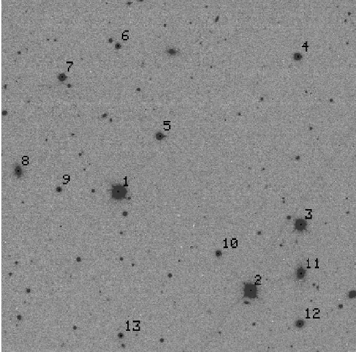
Fig. 1 Observed field. This finding chart was generated by aligning and adding all the images acquired during the second night of observation. The calibrated UBV (RI)c magnitudes of the marked stars can be found in Table 1.
Table 1 UBV (RI)C and 2mass magnitudes of the field stars. Ids as in Figure 1
| ID | Name | RA (2000) | DEC (2000) | U | B | V | Rc | Ic | J | H | Ks |
| 1 | LX Leo | 147.615528 | 20.718239 | 13.581 | 13.102 | 12.212 | 11.678 | 11.164 | 10.591 | 10.081 | 9.985 |
| 2 | 2MASSJ09501501+2040529 | 147.562515 | 20.681321 | 13.695 | 13.307 | 12.466 | 11.982 | 11.511 | 10.787 | 10.336 | 10.231 |
| 3 | 2MASSJ09501021+2042218 | 147.542481 | 20.706063 | 13.990 | 13.978 | 13.371 | 12.992 | 12.639 | 12.125 | 11.796 | 11.733 |
| 4 | 2MASSJ09501054+2046089 | 147.543870 | 20.769125 | 16.724 | 16.013 | 15.062 | 14.488 | 13.959 | 13.226 | 12.699 | 12.605 |
| 5 | 2MASSJ09502379+2044205 | 147.599121 | 20.739021 | 16.069 | 15.886 | 15.143 | 14.719 | 14.306 | 13.738 | 13.331 | 13.224 |
| 6 | 2MASSJ09502783+2046222 | 147.615949 | 20.772882 | 18.955 | 17.762 | 16.337 | 15.451 | 14.564 | 13.607 | 12.978 | 12.768 |
| 7 | 2MASSJ09503319+2045397 | 147.638310 | 20.761087 | 15.547 | 15.660 | 15.252 | 14.991 | 14.726 | 14.391 | - | - |
| 8 | 2MASSJ09503741+2043323 | 147.655932 | 20.725753 | 19.327 | 18.995 | 17.733 | 17.225 | 16.569 | 15.356 | 14.721 | 14.357 |
| 9 | 2MASSJ09503347+2043077 | 147.639424 | 20.718858 | 18.432 | 17.884 | 16.977 | 16.419 | 15.918 | 15.246 | 14.587 | 14.523 |
| 10 | 2MASSJ09501813+2041421 | 147.575551 | 20.695019 | 17.718 | 17.022 | 16.100 | 15.580 | 15.124 | 14.428 | 13.998 | 13.796 |
| 11 | 2MASSJ09501015+2041155 | 147.542298 | 20.687675 | 19.371 | 18.875 | 17.528 | 16.960 | 16.280 | 14.989 | 14.282 | 13.819 |
| 12 | 2MASSJ09501021+2040073 | 147.542536 | 20.668759 | 19.415 | 19.047 | 17.674 | 17.063 | 16.396 | 15.134 | 14.433 | 13.999 |
| 13 | 2MASSJ09502746+2039505 | 147.614426 | 20.664050 | 19.686 | 18.424 | 16.899 | 15.940 | 14.509 | 13.281 | 12.626 | 12.376 |
3. LIGHT ELEMENTS AND (O − C) ANALYSIS
Because the orbital period of LX Leo is important for the rest of the calculations, we tried to refine its value by using our observations and the data found in the literature.
With our observations, and the software package Minima25c (Nelson 2005), times of light minima were calculated as the error weighted average of the values found by the different methods implemented. A total of 6 times of primary and 3 of secondary light minima were calculated and are given in Table 2.
Table 2 Observed times of minimum
| Date | HJD(2400000+) | Error ± | Filter | Type |
| 03.23.2016 | 57470.74662 | 0.00004 | B | I |
| 57470.74660 | 0.00003 | V | I | |
| 57470.74648 | 0.00003 | R | I | |
| 04.05.2016 | 57512.73798 | 0.00005 | B | II |
| 57512.73799 | 0.00004 | V | II | |
| 57512.73806 | 0.00004 | R | II | |
| 06.05.2016 | 57514.73777 | 0.00003 | B | I |
| 57514.73770 | 0.00005 | V | I | |
| 57514.73777 | 0.00004 | R | I |
Another time of minimum is given by Diethelm (2010) as HJD(Min.II) = 2455259.8832(2) (an ephemeris of HJD(Min.I) = 2454918.653 + 0 d .235248 × E is also reported). Additionally, we obtained more times of light minima by fitting our theoretical light curves to the ASAS and Catalina Sky Survey data, adjusting simultaneously in magnitude and time. Because of the highly scattered and sparse survey data, these times of light minima are not as good as those in Table 2 and we estimated that their errors are about 0.005 days. Also, by using the light elements by Diethelm (2010), we obtained the (O −C) diagram shown in Figure 2. The small dots correspond to the values obtained by the light curve fitting method. Using these times of light minima, we applied a weighted linear fit to the data getting a revised ephemeris of
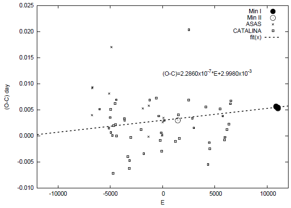
where the values in parentheses indicate the uncertainty in the last digit, and E is the epoch. This improved ephemeris was used in the rest of the calculations of this study. Because of the limited number of times of minima and the small time spans, we were able to do only a linear fit on the (O−C) variation.
4. PHOTOMETRIC CURVES
In Figure 3, all the observations are plotted with respect to our new light elements.
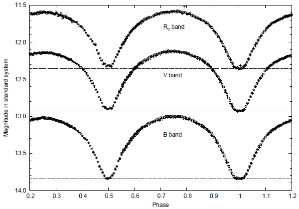
Fig. 3 Phase folded BVR c light curves of LX Leo. Horizontal lines are plotted to highlight the difference between the minima.
As can be seen, there is a total eclipse during the primary minimum. The secondary minimum also becomes almost flat except for a small curvature that can be attributed to limb darkening of the eclipsed component. For systems which undergo complete eclipse, the derived orbital elements are much more reliable. Since one of the components is totally eclipsed, we can determine the real magnitudes of the eclipsing and eclipsed components. Additionally, since the depths of the primary and secondary minima are the same for the B filter and only differ slightly for the V and R c filters, we can say with certainty that the temperatures of the components must be nearly equal. It is important to note that, for light curves that show complete eclipses, the photometric mass ratios are usually very consistent with those obtained spectroscopically (Terrell & Wilson 2005).
The magnitudes at different phases, and the associated colors, are given in Table 3. The difference in depth of the primary and secondary minima is nearly zero for the B filter and becomes larger for longer wavelengths. The differences are 0 m .003 ± 0.009, 0 m .028 ± 0.011 and 0 m .029 ± 0.016 for the B, V, and R c curves, respectively. Furthermore, the primary maximum is lower than the secondary one, the differences being 0 m .021±0.011, 0 m .017±0.007 and 0 m .010 ± 0.007 for the B, V, and R c curves respectively. This type of variations are due to the O’Connell (1951) effect which can be explained by a hot, or cool, spot on one of the components.
Table 3 Magnitudes and colors of lx leo at different phases
| Phase | B±σ | V±σ | R c ±σ | (B-V)±σ | (V-R c )±σ |
| 0.00 | 13.839±0.007 | 12.924±0.005 | 12.347±0.014 | 0.915±0.009 | 0.577±0.015 |
| 0.25 | 13.018±0.005 | 12.141±0.003 | 11.595±0.006 | 0.877±0.006 | 0.546±0.006 |
| 0.50 | 13.835±0.005 | 12.896±0.009 | 12.318±0.007 | 0.939±0.011 | 0.578±0.012 |
| 0.75 | 12.997±0.010 | 12.124±0.006 | 11.586±0.004 | 0.873±0.011 | 0.538±0.007 |
Except during primary minima, most of the W UMa-type systems show small color changes with respect to the orbital phase. It can be seen, Figure 4, that the variations of colors (B − V ) and (V − R c ) are no larger than 0 m .04 and that there is a small color difference between both minima. Because the color (B−V ) at the primary minimum is a bit lower than at the secondary minimum, at this phase, we can say that the cooler component is eclipsed by the hotter one. But this is not seen for the (V − R c ) color. If this is true, the cooler component must be larger than the hotter one and the primary minima must show an annular eclipse. Because the color differences between primary and secondary minima are small, ∼ 0 m .024, it is possible that the eclipsing component at the primary minimum has a hot spot on its surface, making the system bluer during this phase.
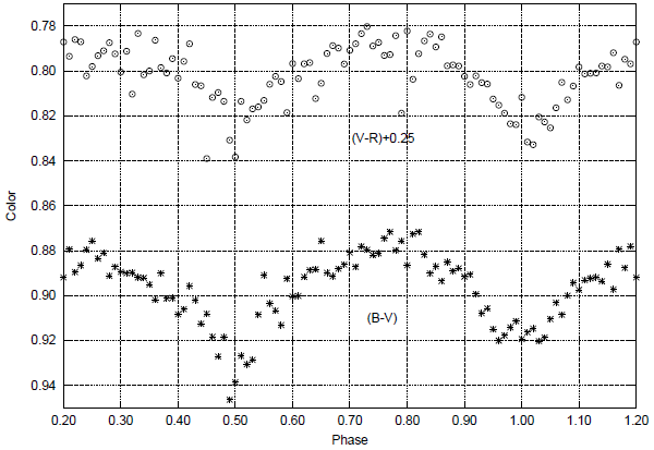
Fig. 4 The observed color curves of LX Leo. The color values correspond to the difference of the averaged magnitudes over 0.01 phase intervals.
We derived the effective temperature of the system from the colors at specific phases. In Table 4 we list the colors and their corresponding temperatures using the color-temperature relations and tables given by Cox (1999), Pecaut & Mamajek (2013), Houdashelt et al. (2000) and Collier et al. (2007). Except for the temperatures obtained for the (V − R c ) color, at primary minimum the hotter component is in front of the cooler one and its mean temperature is 4908K. The temperatures from JHK colors, which correspond to orbital phase 0.4 when the cooler component is partially in front of the hotter one, imply a mean temperature of 4913K which agrees with the previous one.
Table 4 Colors and temperatures of lx leo at specific phases
| Phase | Color(mag.) | Cox (1999) | Pecaut & Mamajek (2013) | Houdashelt et al. (2000) | Collier et al. (2007)) |
| (oK) | (oK) | (oK) | (oK) | ||
| 0.00 | (B-V)=0.915 | 4821 | 4995 | 4909 | - |
| 0.00 | (V-Rc)=0.577 | 5329 | 4764 | 4774 | - |
| 0.40 | (H-K)=0.096 | 4875 | - | 4812 | - |
| 0.40 | (J-K)=0.606 | 4938 | - | 4937 | - |
| 0.40 | (J-H)=0.410 | 4954 | - | - | 4960 |
We should expect lower temperatures if the light is highly affected by interstellar reddening but this can not be clearly seen in Table 4. This is possible if the eclipsing system is not far away from us. But if the distance given by is true, the system must be affected by interstellar dust and gas and, as a result, appear redder at shorter wavelengths. Since the distances of stars determined by were obtained by using calibrations of absolute magnitudes of single main-sequence stars, they are probably not appropriate for contact binaries. As can be seen in the color curves of Figure 4, the amplitude of the colors does not change more than 0m.04 and we can accept that the lower limit of the primary’s temperature is around 4900K.
In principle we do not have any information about the reddening of the system, but it cannot be very large because of the high galactic latitude (+48◦). According to the extinction maps2 of Schlegel et al. (1998), the total extinction in the direction of LX Leo is A v = 0.06−0.07. Because these values are given for an infinite distance, the reddening of the system must be smaller. An estimation of reddening can be done, by using total extinction and distance to the system, with the 3rd equation of Bilir et al. (2008). Assuming the distance to the system given by Pickles & Depagne (2010), the resulting reddening is about 0 m .06, while the corresponding color excess is E(B − V ) = 0.06/3.1 ∼ 0.02.
Additionally, the period-color relation given by Wang (1994) (based on the assumption that the components in a contact binary system are formed from almost normal hydrogen-core-burning stars that obey the mass-radius relation for main sequence stars) predicts that the intrinsic color index can be written as
where P is the orbital period in days. For this equation, the correlation coefficient to the fit given by Wang (1994) is 0.80. Using the period obtained in this work, we derive the intrinsic color of the system as (B − V )0 = 0 m .885. The color excess obtained by the difference between the intrinsic and the observed color at phase 0.0 is E(B − V ) = 0.03 which agrees with the previously obtained value. The corresponding temperatures and spectral types are 4909K (K1V/K2V) (Cox 1999), 5062K (K1V/K2V) (Pecaut & Mamajek 2013) and 5053K (Houdashelt et al. 2000). The average of these temperatures is 5008±86K and differs by nearly 100K from the values obtained by using the observed colors. Using the color excess value (∼ 0.02) and the (B − V) colors given in Table 3 for different phases, the average temperature is 5073 ± 75K which is not much different from the previous one. The accepted temperature of the hotter component in the light curve analysis is 5050 ± 100K.
5. LIGHT CURVE ANALYSIS
Because there is a clear indication of the O’Connell effect, we first want to predict some parameters about the spot, or spots, located on one of the components. For this prediction we fold the first half of the light curves over the second half as shown in Figure 5. As can be seen, around the primary and secondary minima, the spot or spots do not affect the light curves. The variation is mostly seen between phases 0.10 and 0.38 for a cool spot or spots, or between 0.62 and 0.90 for a hot spot or spots. The variation is no larger than 0m.03 in the B band and becomes smaller for longer wavelengths. This implies that the spot’s temperature factor must be small.
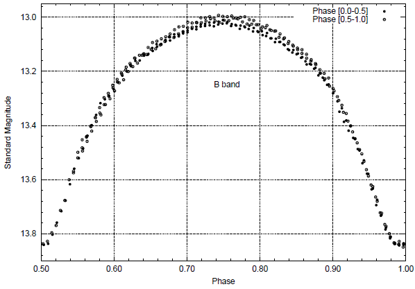
Fig. 5 Folded B light curves of LX Leo with respect to the secondary minima. The O’Connell effect is mostly seen between 0.62 and 0.90 or between 0.10 and 0.38 orbital phases. The effect decreases at longer wavelengths.
The spot affects ∼ 28% of the light curves. Assuming the spot is located on the equator, its angular radius can be as large as ∼ 50◦. It is also possible that the spot is located away from the equator and can be seen over a large phase interval. Additionally because of the duality between the spot angular radius and temperature factor it is possible that the same effect can be produced with a smaller and hotter spot (or spots). Because of these restrictions the location, angular radius, and temperature factor of the spot (or spots) can only be assumed parameters.
If we assume that the center of the O’Connell effect occurred at orbital phases of 0.24 (for a cool spot) or 0.76 (for a hot spot) we can obtain the longitude of the spot’s center as 86◦ .4 or 273◦ .6, respectively. Because there is no clear indication of any discrete (pieced) spot structure in this interval, we can say that the effect is most likely produced by a single spot. The activity vanishes at longer wavelengths, especially for R c where we can hardly see the effect on the light curves (see Figure 7). The fact that the color amplitude decreases towards longer wavelengths suggests that the spot is hotter than the surrounding surface (Kallrath & Milone 1999).
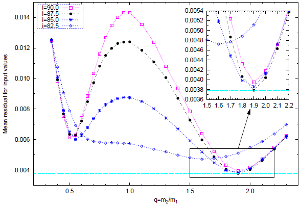
Fig. 6 [i,q] search of LX Leo. Mean residuals for input values as function of the mass ratio and orbital inclination. The i − q search method was implemented by taking i and q as constant and then varying the other parameters, on Mode 3, to find the lowest values of the residuals.
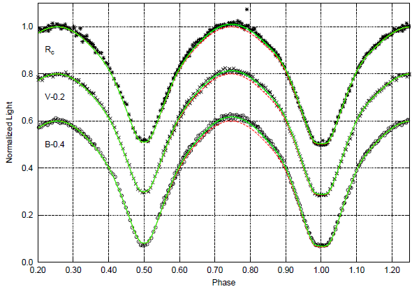
Fig. 7 The observational and theoretical light curves of LX Leo. The symbols represent the observational data for the BVRc filters and the lines the theoretical light curves for over-contact mode with (continuous) and without (dashed) hot spot located on the secondary component.
The Wilson & Devinney method (Wilson & Devinney 1971; Wilson 1979, 1990; Wilson & van Hamme 2007) was applied to solve the light curves of LX Leo as in our previous paper (Gürol & Michel 2017). The subscripts 1 and 2 refer to the primary (hotter) and the secondary (cooler) component, respectively.
In all our solutions, we have set the temperature of the hotter component to T1 = 5050K (as obtained in the previous section). The spectral type that matches this temperature is K1V according to the tables by Cox (1999) for main sequence stars. The linear bolometric and logarithmic darkening coefficients were taken from van Hamme (1993). Because of the convective atmospheres, the gravity darkening exponents and the bolometric albedos were set to 0.32 (Lucy 1967) and 0.50 (Rucinski 1969), respectively, for both components. Circular orbit and synchronous rotation were assumed. No third light was allowed for, hence l 3 = 0.00. These parameters were kept constant during all the iterations.
For our solutions we assumed that the system is in contact, by employing the Mode 3 option of the code (over-contact mode). The adjustable parameters were: the inclination i, the mean surface temperature of the secondary component T 2, the nondimensional surface potential of the primary component Ω1, and the monochromatic luminosity of the primary component L 1. We selected IPB=0; thus, the temperature of the secondary component was used to calculate the L 2 values.
Due to the lack of information on radial velocity, the orbital semi-major axis was estimated using the P − ɑ calibration by Dimitrow & Kjurkchieva (2015); we obtained ɑ[R ⊙] = 1.72 ± 0.05.
Since we see traces of a hot spot on one of the components, we must first obtain a crucial solution using preliminary starting parameters. In order to achieve this, we selected a starting point using a q-mass ratio of 0.5 and we located a hot spot on the secondary component. The spot could also have been located on the primary component but, since the spot modeling is not unique, we simply chose the spot to be on the secondary star as a possible model, and not necessarily the reality. By using the method for modeling such spotted light curves given by Gürol (2005b), who firstly obtained the light curve solution for the unaffected portion of the light curves and then solved the entire light curves by including the spot parameters, we obtained preliminary geometric parameters of the system for the rest of the calculation.
Since no spectroscopic mass ratio and inclination are available, the [i − q]-search method was applied for a mass-ratio q ranging from 0.35 to 2.30 and an inclination i ranging from 82◦ .5 to 90◦. We started the [i−q]-search by taking i and q constant and setting T 2, Ω, L 1, and the temperature factor of spot as free parameters. The results are given in Figure 6. Mean residuals were defined as the sum of the weighted squared residuals divided by the number of observations (private communication with Wilson, R.E.). As can be seen, the best solution was reached when i = 87◦ .5 and q phot = 1.90. This parameters indicate a W-type W UMa system, i.e., the smaller, less massive component has the higher surface temperature but contributes less to the overall brightness of the binary as a whole because the larger star contributes more to the luminosity due to its larger surface area.
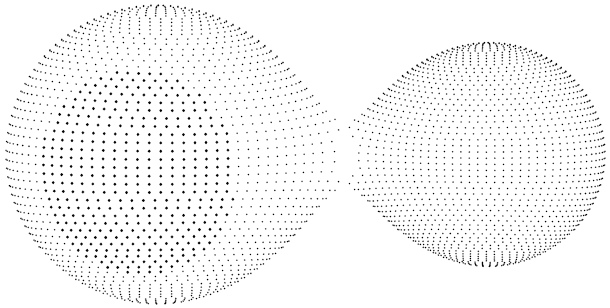
By using the initial parameters (T 1, q phot , i and spot parameters) as input values we solved the light curves until the solution converged. The convergent solution was obtained with the adjustable parameters by iterating, until the correction on the parameters became smaller than the corresponding standard deviations. The observed and theoretical light curves, calculated with the final elements, are shown in Figure 7 and the residuals of the fit with the observations in Figure 8. The results of the final solution are given in Table 5 including the standard deviation of the parameters calculated by solving individual light curves. The configuration of LX Leo calculated with the Roche model is shown in Figure 9.

Table 5 The light curve solutions of LX LEO*
| Parameter | BV R c | ±σ |
| α(R ⊙) | 1.72∗ | 0.05 |
| i(o) | 86.7 | 0.6 |
| q = m2/m1 | 1.89 | 0.02 |
| T 1(K) | 5050∗ | 100∗ |
| T 2(K) | 4916 | 18 |
| A 1 = A2 | 0.50∗ | - |
| g 1 = g2 | 0.32∗ | - |
| x 1(bolo) | 0.641∗ | - |
| x 2(bolo) | 0.636∗ | - |
| y 1(bolo) | 0.168∗ | - |
| y 2(bolo) | 0.156∗ | - |
| Ω1 = Ω2 | 4.999 | 0.026 |
| Ω in | 5.089 | 0.025 |
| Ωout | 4.193 | 0.019 |
| Fillout:f 1 = f 2 | 10.0% | 0.4 |
| L 1 /L Tot. (B) | 0.4080 | 0.0008 |
| (V ) | 0.3984 | 0.0007 |
| (R c ) | 0.3910 | 0.0006 |
| L 2 /L Tot. (B) | 0.5920 | - |
| (V ) | 0.6016 | - |
| (R c ) | 0.6090 | - |
| r 1(pole) | 0.3125 | 0.0009 |
| r 1(side) | 0.3276 | 0.0010 |
| r 1(back) | 0.3654 | 0.0011 |
| r 2(pole) | 0.4170 | 0.0007 |
| r 2(side) | 0.4440 | 0.0008 |
| r 2(back) | 0.4754 | 0.0008 |
| σ B | 0.0073** | - |
| σ V | 0.0067** | - |
| σ Rc | 0.0070** | - |
| Secondary Component | ||
| Spot co-latitude(◦)= | 96; | 3 |
| Spot longitude(◦)= | 258; | 10 |
| Spot radius(◦)= | 42.4; | 0.7 |
| Spot temp.factor= | 1.0079; | 0.0010 |
* Assumed parameters are marked with ∗ and standard deviations for computation of curve-dependent weights with ∗∗. The errors given here correspond to the standard deviations of the calculated parameters.
6. ABSOLUTE PARAMETERS
Using the semi-major axis of the orbit obtained previously and the orbital period, P = 0 d .2352482(3), we calculated the system’s total mass as 1.23 ± 0.11M ⊙. Since the mass ratio of the system was found to be q = m2/m1 = 1.89 ± 0.02, we derived the masses of the primary and secondary components as M 1 = (0.43 ± 0.04)M ⊙ and M 2 = (0.81 ± 0.07)M ⊙, respectively.
With the semi-major axis and the mean fractional radii given by the light curve solution we found the radii of the components which are R 1 = (0.58±0.02)R ⊙ and R 2 = (0.77±0.02)R ⊙. Because the sum of the mean fractional radii of the components is r mean = 0.78 > 0.75 the system is in a state of marginal contact (Kopal 1959).
Knowing the radii and temperatures of the components, the calculated bolometric magnitudes are M bol1 = 6.54 ± 0.11 and M bol2 = 6.03 ± 0.07, and the luminosities are L 1 = (0.19 ± 0.02)L ⊙ and L 2 = (0.31 ± 0.02)L ⊙. According to the equations given by Mochnacki (1981), the mean densities of the components are ρ 1 = 3.16 ± 0.02 g cm−3 and ρ 2 = 2.54 ± 0.02 g cm−3.
With the period-luminosity-color relation for contact binaries given by ,
we can obtain the absolute magnitude of LX Leo using the orbital period (P in days) and intrinsic color of the system with the error of ±0.25. By using (B−V )0 = 0.877−0.02 = 0.857 and system’s orbital period, the absolute magnitude of the system turns out to be M V = 5.50±0.25. Since the V magnitude of the system is 12.141± 0.003, we find the distance modulus of the system to be V − M V = 6.64 ± 0.25 giving a distance to the system of 207 ± 25 pc. In Table 6 we present the absolute parameters of the eclipsing binary system LX Leo. The location of the components of LX Leo on the log T −log L diagram is given in Figure 10, including other W- and A-type W UMa systems from the list of Yakut & Eggleton (2005) and from the works of Gürol and Gürol et al. (Gürol & Müyesseroglu 2005a; Gürol 2005b; Gürol et al. 2011a,b, 2015a,b,c, 2016a; Gürol 2016b; Gürol & Michel 2017). As can be seen, the primary component is located within the main-sequence while the secondary component is located below it, consistent with the other W-type systems.
Table 6 Absolute parameters of LX LEO
| Parameter | Primary | Secondary |
| Mass (M ⊙) | 0.43 ± 0.04 | 0.81 ± 0.07 |
| Radius (R ⊙) | 0.58 ± 0.02 | 0.77 ± 0.02 |
| Luminosity (L ⊙) | 0.19 ± 0.02 | 0.31 ± 0.02 |
| M bol | 6.54 ± 0.11 | 6.03 ± 0.07 |
| Log g (cgs) | 4.55 ± 0.05 | 4.58 ± 0.05 |
| ρ(g cm−3) | 3.16 ± 0.02 | 2.54 ± 0.02 |
| ɑ(R ⊙) | 1.72 ± 0.05 | |
| d(pc) | 207 ± 25 |
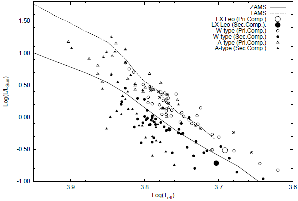
Fig. 10 The location of the components of LX Leo in the logT−logL diagram. Open symbols for primary and full symbols denote the secondaries. The sample of Wand A-type systems are from Yakut & Eggleton (2005) and from the works of Gürol et al. (see text). The lines shown are for solar-metallicity, ZAMS (lower) and TAMS (upper) from Girardi et al. (2000).
7. RESULTS AND DISCUSSION
We have derived, for the first time, a photometric solution for the eclipsing binary system LX Leo. We found that this binary is a W-type over-contact system with a mass ratio of q = 1.89 ± 0.02, and a shallow degree of physical contact (f = (Ω in − Ω)/(Ω in − Ω out ) = 10%) including thermal contact between components (∆T ∼ 134K). The photometric mass ratio found in this work can only be confirmed by spectroscopic observations, but as can be seen in several works (Lapasset 1992; Maceroni and van’t Veer 1996; Terrell & Wilson 2005) the photometric and spectroscopic mass ratios are very consistent with each other for W UMa type systems showing total eclipse.
Because of restricted time span of times of light minima we cannot say much about the period variation of the system, but with the available data we refined the light elements and used them in this analysis. We found that the light curves showed a decreasing O’Connell effect toward longer wavelengths, which we assume is produced by a hot spot located on the secondary component with a small temperature factor. The corresponding spectral types for the components are approximately K0V + K1V for the primary and secondary, respectively.
Absolute parameters were obtained by using the empirical relation given for W UMa type systems by Dimitrow & Kjurkchieva (2015); the uncertainties of the parameters are relatively small.
Overcontact systems are important objects in astrophysics, especially for understanding the very late evolutionary stages of the binaries connected with the processes of mass and angular momentum loss, merging or fusion of the stars, etc.

