1. Introduction

This is the first of a series of works in which we intend to deal with different optical phenomena taking place in planetary atmospheres. We will begin by addressing the study of some phenomena related to light refraction that are known to occur in the Earth’s atmosphere. The refraction of light in the Earth’s atmosphere is a topic of great interest to astronomers, geophysicists, and meteorologists. Refraction is an unavoidable issue whenever we are dealing with the propagation of radiation through the terrestrial atmosphere, in relation to the image formation of either astronomical or terrestrial sources, or in relation to radio communication and radar systems. At the first works we will focus on image formation.

Regarding the study of refraction for astronomical purposes, more or less complete treatments appear in general or spherical astronomy textbooks as old as Danjon (1959)¹. Mahan (1962)², Garfinkel (1967)³, and Yatsenko (1995)⁴, just to name a few, have published on astronomical refraction. Many publications proposing new approaches and formulas for the calculation of refraction, in particular near the horizon, are found in the literature. A very valuable contribution has been made by Young (2006)⁵, who focuses on the physics of refraction beyond formulas and numerical calculations. Many authors have, also, studied in detail the influence of refraction in observations of the sun (Corbard et al., 2019⁶).

In the present paper we deal with image formation of terrestrial sources, particularly, inferior mirages. An inferior mirage is an atmospheric optical phenomenon often seen on summer days on highways and deserts. The soil surface is heated by the sun causing a strong temperature gradient in the air layers closest to the ground.

Several articles referring to the light ray paths through refractive media are found in the literature. Evans and Rosenquist (1986)⁷ and Evans (1990)⁸ presented an original formulation of the theory of light rays in variable refractive index media. From the variational principle, they derived a differential equation for a ray of light similar to Newton’s law of motion for a particle in a conservative force field. In the first of these papers they even solved this equation for the particular case of inferior mirages assuming a linearly varying refractive index. Nener et al. (2003)⁹ found, working in spherical coordinates, an expression describing the ray paths with exact solution for linear and quadratic refractive index profiles. In a later article (Fowkes & Nener, 2005¹), they adopt a refractive index that varies exponentially near the ground and linearly higher up, finding thus two solutions to describe the paths of light rays, the inner and the outer solution.

Many articles based on the ray tracing technique have, also, been published. With this method, so widely used in computer graphics, they created algorithms that allowed them to simulate different optical phenomena (Berger et al., 1990¹¹, Musgrave, 1990¹², Stam and Languenou, 1996¹³, Gutierrez et al., 2006¹⁴).

In this series, we aim to individually analyze each phenomenon related to the refraction of light in the Earth’s atmosphere. This will allow us to make the appropriate considerations in each particular case and thus achieve simpler analytic expressions. Our objective in the present work is to find such an expression describing the path followed by light when an inferior mirage is taking place.

To develop our ideas, we consider a plane-parallel atmosphere assuming that in each layer all the physical parameters characterizing it remain constant. All investigations related to atmospheric conditions that give rise to inferior mirages show that the required temperature inversion occurs very close to the ground. Personal experiences verify it. Only our feet are able to feel the high temperatures of a surface heated by the sun’s rays. The upward heat transport that takes place creates a temperature profile characterized by a sharp 10 - 20 °C drop in a few centimeters of air. When going from a sitting to a standing position, we are not able to notice such a drop in temperature. The departure of the air refractive index from its normal conditions, that will cause the light rays to bend upwards, occurs, then, very close to the ground. The paths of light rays from objects in our environment can be considered straight lines for most of their travel. The distances traveled by light within the layers of air that curve it upward are too short to take into account the earth sphericity. We also assume that the geometrical optics laws apply. A detailed analysis of the validity ranges of this assumption are found in Born & Wolf (1959)¹⁵ and Jackson (1975)¹⁶. Since light travels an optical path that is stationary with respect to variations of that path, the Fermat’s principle is applied in order to compute the path of light.

Our approach to the problem will be correct as long as we are dealing with refractive media in which the refractive index, n, only varies with one coordinate, and the particular solution we found will remain valid provided that the refractive index varies with that coordinate in the exponential way that we propose. The refractive index profile we propose is not, however, a limitation, if what we want to study are inferior mirages. As we will see later, the profile we have adopted for n is the one suggested by both theoretical and experimental research on the subject.

We organize this paper as follows: In Sec. 2 we address the issue of heat transport in the microlayer. In Sec. 3 we study the paths of light rays, dealing with mathematical development that leads us to find the analytic expression we are looking for in Sec. 3.1. Then, a description of the light ray paths and an analysis of the expression obtained is presented in Sec. 3.2. Finally, in Sec. 4 we briefly summarize our results and reach our conclusions.

2. Heat transport

In this section, we aim to find a feasible refractive index profile under the conditions in which mirages occur. Several authors argue that the appropriate atmospheric conditions to produce mirages occur very close to the ground (Stull, 1988¹⁷, Stam and Languenou, 1996¹³). Solar radiation heats the surface of the road raising its temperature well above the air temperature, which causes upward heat transport by molecular and turbulent processes through the microlayer. We do not intend to work out a detailed profile of the parameters that describe the atmosphere, but just to find the way in which, under given conditions, the air temperature in the microlayer decreases with height. A rigorous treatment of the energy balance taking into account downwards and upwards radiation is not justified, neither a detailed approach to convection. The way we have dealt the heat transport through the microlayer will be explained in the following paragraphs.

We write the heat flux across the microlayer, Q, as the sum of two terms

being Q_c and C_t the heat transported by molecular and turbulent processes, respectively.

By setting the origin of the Cartesian coordinate system on the ground and the y-coordinate axis perpendicular to it, the heat transported by conduction can be written as

being κ the thermal conductivity of air. To take into account the temperature dependence of κ we use the expression of Kannuluik and Carman (1951)¹⁸,

where [T] = °C and [κ] = Cal/°C cm s.

Regarding convective transport, we made the following assumptions: i) we only took into account turbulent flux, since the vertical advective flux is negligible compared to the turbulent one (Stull, 1988¹⁷) and we are only interested in upward heat flux, and ii) under the constraint of total heat flux conservation, we express turbulent flux as a fraction ƒ of the molecular one, taking into account that conduction dominates very close to the ground, decreasing with the height as turbulence increases. Therefore Eq. (1) can be written as

Taking into account the κ dependence on T given by Eq. (3), we integrate both members of the expression (4) and iteratively solve it to find the variation of temperature with height from the ground. The total heat flux, Q, and the ground temperature, T₀, are parameters adopted at the beginning. Although Q and T₀ are not actually independent parameters of each other, they are not unambiguously related; their relationship depends on the kind of surface. Taking them as unrelated parameters allows us to observe the influence of each one on the results, not affecting our conclusions at all. We have done calculations by making ƒ vary with height in different ways. The way ƒ varies with height determines the height from the ground at which the molecular and turbulent processes are of the same magnitude. That height in turn determines how quickly the temperature drops and, thus, the T_ƒ environment temperature reached away from the ground. Working in this way, we achieve results like those shown in Figs. 1, 2 and 3.

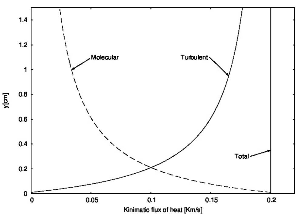
Figure 1 Heat transport. A solid line shows the turbulent heat flux, and a dashed line shows the molecular heat one. The total flux, equivalent to 200 W/m2, is also indicated. 

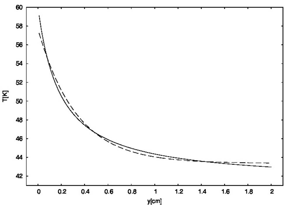
Figure 2 Temperature profile. A solid line shows the atmospheric temperature profile near the ground obtained from our calculations, and a dashed line shows the fitted exponential function. 

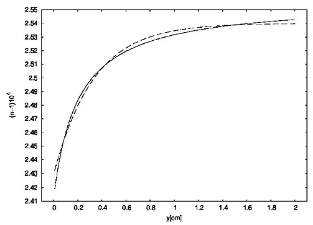
Figure 3 Refractive index profile. A solid line shows the refractive index profile of the air close to the ground gotten from our calculations, and a dashed line shows the fitted exponential function. 

In Fig. 1, where the heat transported by molecular and turbulent processes as functions of height are drawn, we have managed to obtain a diagram similar to the one shownin Fig. 7.1b) of Stull (1988)¹⁷ assuming Q = 260 W/m² (equivalent to a kinematic heat flux Q/ρCp = 02 Km/s as it is expressed by Stull, 1988¹⁷).

Although we are not particularly interested in the course of the heat fluxes through the microlayer, this figure is useful just to check that the way we have modeled the heat transport mechanisms makes things go reasonably well. As can be seen in the figure, the turbulent heat transport takes on the same importance as the molecular one at 2 mm from the ground.

Assuming T₀ = 60, the temperature profile through the microlayer, displayed with solid line in Fig. 2, is obtained.

Its sharp drop in the lowest millimeters of air is apparent. It is also clear that the temperature as a function of height can be adjusted with an exponential function like

where ∈ = T₀/T_ƒ - 1 is obtained by setting y = 0 in Eq. (6), and h₀ is a positive constant to be determined in each particular case. So, in terms of T₀ and T_ƒ the temperature as a function of height can be written as

The dashed curve displayed in Fig. 2 is obtained for h₀ = 0.33 cm. Such a sudden exponential drop in temperature very close to the ground in the context of mirages sighting has already been argued by several authors (Stull, 1988¹⁷, Stam and Languenou, 1996¹³).

To obtain n as a function of height we take into account that it can be written so that

where δ is the refractivity for atmospheric pressure P = 76 cmHg and temperature t = 0, and D is the pressure and temperature correction factor. Both, δ and D, are dimensionless parameters.

To take into account the δ dependence on the wavelength of light we have used the Ciddor (1996)¹⁹ formula

given for t = 15, P = 76 cmHg, and 0% humidity, with λ in microns.

The factor D can be writen as

with P in cmHg and t in °C.

Assuming t = 15 and P = 76 cmHg for the calculation of D in Eq. (7) and equating to Eq. (8), δ can be calculated for any λ value as

Then, n can be obtained for any t and P values from Eq. (7).

Then, by setting P = 76 cmHg, and adopting the temperature profile shown in Fig. 2, we have obtained the refractive index as a function of height for λ = 0.5 µm, as shown with solid line in Fig. 3.

Given the n dependence on T, it is clear that the variation with the y-coordinate of the refractive index calculated for a temperature profile given by Eq. (6), can be fitted with a function like

being n_ƒ the n value far from the ground, where the temperature has reached the environment value T_ƒ. α and β are positive constants to be determined in each particular case, that is, for each particular temperature profile. The best fit to our calculations is obtained by setting n_ƒ = 1.00025, α = 1.10865(10^-5 and β = 0.33 in Eq. (12), as we show with the dashed line in Fig. 3. Since α = 1 - n₀/n_ƒ is obtained by setting y = 0 in Eq. (12), where n₀ is the n value on the surface, n can be written in terms of n₀ and n_ƒ as

Then, we can also use the n_ƒ and n₀ values that we got from the calculations and only look for the β value that provides the best fit. The setting varies slightly.

We have made calculations varying Q, T₀ and the way ƒ varies with height. Q was varied between 200 W/m² and 500 W/m² and T₀ between 40 °C and 70 °C, as theoretical simulations and empirical measurements suggest (Garrat, 1991²⁰, Heusinkveld, 2008²¹, Pfeiffer, 2021²²), although T₀ higher than 70 °C in unusual extreme conditions could occur. As for ƒ, it is worth noting that the thicker the atmosphere layer in which molecular processes take place, the faster the temperature falls. Therefore, we have modeled ƒ in such a way to achieve 𝑇 𝑓 values between 40 and 20. We have limited ourselves to these T_ƒ values since, except for very extreme conditions, the room temperature on days in which an inferior mirage could be observed will fluctuate between these values. For these T_ƒ values, the height from the ground at which the molecular and turbulent processes are of the same magnitude has varied between 1 and 7 mm.

We have been able to verify that, for those parameter ranges, α varies between 1.1x10^-5 and 4x10^-5, β ranges from 0.3 to 0.8 cm. Given the dependence on T of n, and taking into account the smallness of δx10^-6, it is clear that β and h₀ will always be very similar.

3. Path of light rays.

3.2. Description and analysis.

Light rays leaving a point object start its way towards the ground following different directions. Some rays reach the ground being absorbed by it. Others are refracted upward before reaching the ground. Whether one thing or the other happens depends on the angle that the ray coming from the object makes with the ground, which is assumed to be horizontal. There is a limiting angle, which we will call θ, for which the ray will barely touch the ground before continuing its way up. If the rays leave the object forming angles larger than θ with the ground, they will be absorbed by the ground, otherwise the rays will bend upward before reaching it. The distance from the object at which a ray hits the ground or reaches its minimum height also depends on that angle. This behavior of the rays is illustrated in Fig. 4, where the height from the ground, y, as a function of the distance to the object, d, is displayed.

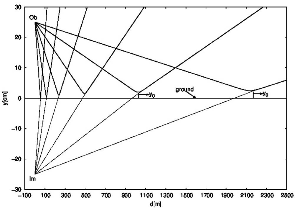
Figure 4 Light ray paths. The height from the ground is displayed as a function of the distance to the object for some rays. The object point from which the light comes and its virtual image are also shown. 

Figure 4 was drawn up by means of Eq. (23), adopting α = 1.10865x10^-5 and β = 0.33, the values that we used in Sec. 2 to fit our calculations. We should note that Eq. (23) was achieved by setting x = 0 at y = y₀ for each ray. Then, in order to refer everything to the same point, we have calculated the shift of every ray with respect to each other by imposing that they all pass through the same point object. So, to be clear: x is 0 at the point of closest approach to the ground of each ray; d is 0 at the point object. The virtual image of a hypothetical point object located 25 cm above the ground is also shown in the figure.

Figure 5 shows an enlarged image of some light paths, just to observe their behavior around the point (0,y₀), which will be called “V point” from now on. Straight dashed lines represent the asymptotic approach of the light ray paths. These straight lines are given by the equation

y=1γx-βln4+y0, (24)

which is easily obtained from Eq. (23) taking into account that the exponential tends to 0 when y takes very large values. As can be seen from the figure, the curves representing the light ray paths approach very quickly to their asymptotes as we move away from V point, being confused with them a few millimeters further.

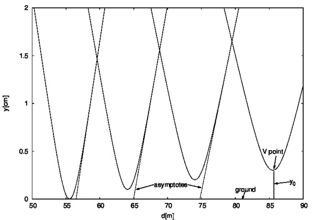
Figure 5 Light ray paths close to V points. Enlarged image of some light rays around V points (see text) and their asymptotes are shown. 

Before we go any further, we take advantage of Eq. (24) to obtain an expression for the limiting angle, which we referred to above, that allows to distinguish the light rays absorbed by the ground from those refracted upwards. The angle that the ray coming from the object makes with the ground is just the angle that its asymptote makes. So, to find the limiting angle we simply have to find the slope of the asymptote to the ray that barely touch the ground for which y₀ = 0. Then, by setting y₀ = 0 in Eq. (24), and taking into account that α << 1, θ is obtained as

θ=arctan(2α) (25)

From Figs. 4 and 5 it appears that the light paths through the atmosphere given by Eq. (23) are practically straight lines from the object to very close to the point where they are bent upward to eventually reach the observer’s eyes. In other words, inferior mirages like the ones we are studying in the present article are due to what happens around V points.

Equation (23), in addition to the description of the light ray’s path, is a source of much relevant information. We will use it below to learn about the height from the ground at which the right conditions for an inferior mirage to occur are met. Since everything happens around V points, we could get our objective by estimating the y₀ values of the rays that could reach the observer’s eyes. In order to do that, letting y₀ vary in Eq. (23) we have calculated x for picked y values. The y values we have chosen to do the calculations, which will be called y_0b hereafter, are some feasible values of the height from the ground at which the observer’s eyes could be. To draw Fig. 6, the calculated x values have then been referred to a hypothetical object point located at h = 1m from the ground.

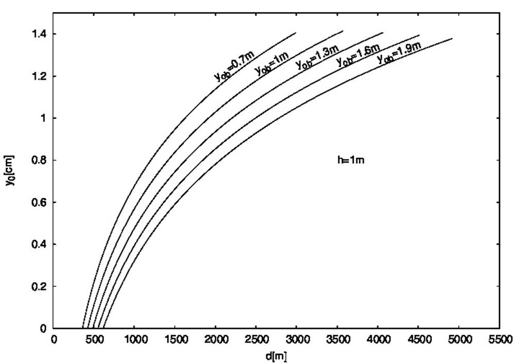
Figure 6 Light rays from a point object reaching the observer’s eyes. The y₀ value of the ray reaching the observer’s eyes, who is at the distance d from the object, is shown for different y_0b values. The point object was assumed to be at h = 1 m above the ground. 

Each point of a given curve in Fig. 6 represents the y₀ value of the ray that reaches the observer’s eyes located at the height y_0b from the ground and at the distance d from the object. In Fig. 7, the y₀ value is shown as a function of the distance to the object for different values of h, assuming the observer’s eyes 1m above the ground.

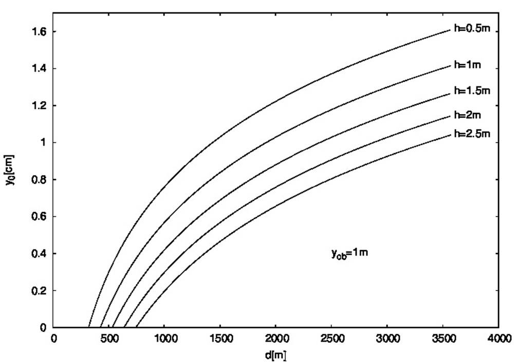
Figure 7 Light rays from different point objects reaching the observer’s eyes. The y₀ value of the ray reaching the observer’s eyes, who is at the distance d from the object, is shown for different h values. The observer’s eyes were assumed to be at y_0b = 1 m above the ground. 

From Figs. 6 and 7 it is clear that rays with different y₀ values will reach the observer’s eyes depending on the distance to the object, which was varied between a minimum and a maximum value. On the one hand, there is a minimum distance to the object, d_min, that the observer should be to witness a mirage, which can be calculated as

dmin=h+yobtan⁡θ=h+yob2α. (26)

Given that α can be obtained from Eq. (12), as we pointed out in Sec 2, and taking into account the dependence of the refractive index on the temperature, d_min can be written in terms of the surface and the environment temperatures. So, writing α in terms of n₀ and n_ƒ, and taking into account Eqs. (7) and (9). Equation (26) can be written as a function of the surface and the environment temperatures as

dmin=h+yob2A(T0-Tf)T0(Tf+A), (27)

where A = δx10^-6 273.

Taking into account the range of variability of the parameters, we can easily do some calculations. The observer, whose eyes are 1m from the ground, should be at a distance greater than 671 m from a 5 m high palm tree to see the image of its tip, and at a distance greater than 113m to see its base. Those values will change to 1280 and 215 m, respectively, for the smallest α values.

On the other hand, and just to impose an upper limit on how far the observer could be to see a mirage, the calculated distance was constrained to be smaller than the distance to the horizon for the adopted y_0b value. The ray with the maximum y₀ value that the observers will be able to see is that reaching their eyes when they are located at the distance of the horizon from the object. This maximum y₀ value, called y^m₀ from now on, is plotted in Fig. 8 as a function of y_0b for different h values.

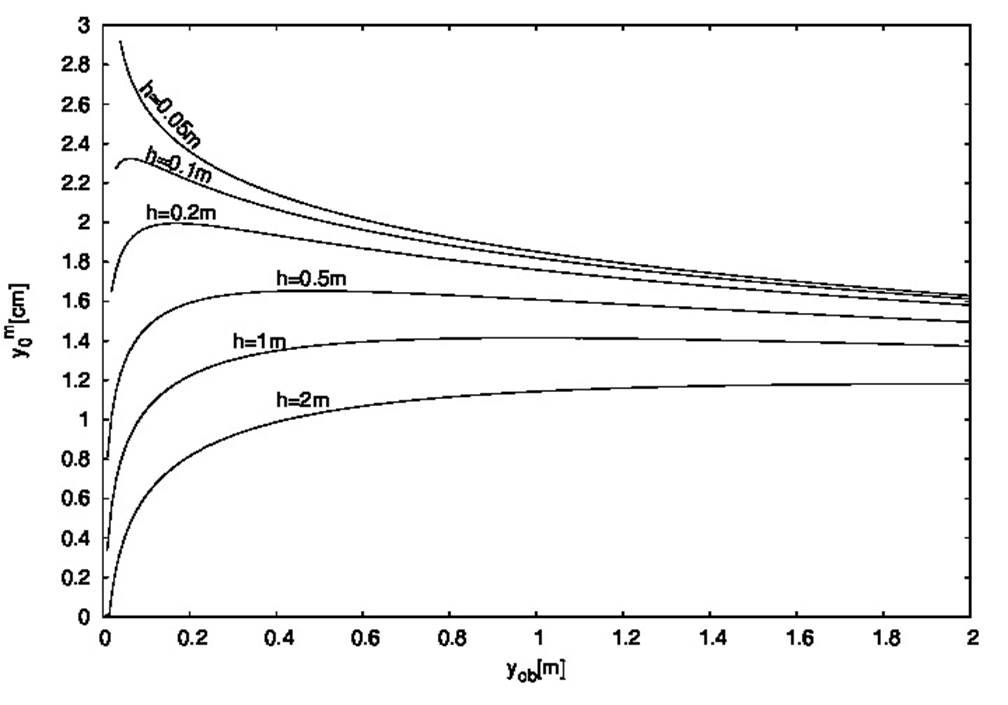
Figure 8 Light rays with the maximum y₀ value reaching the observer’s eyes. y^m₀ is displayed as a function of y_ob for point objects located at different height, h, above the ground. 

In typical situations of sighting of this type of mirages, walking or driving along a paved road, the observer’s eyes are not closer to the ground than 1 m. It is apparent from Figs. 6, 7, and 8 that, for the adopted α and β values, the rays that could reach the observer’s eyes are those characterized with y₀ values smaller than 2 cm. Actually, we can say that rays with y₀ so large hardly reach the observer’s eyes, since these maximum values are reached for very long distances to the object. Rarely is the ground surface flat and unobstructed to allow the observer to simultaneously view the object and its image at such great distances.

For different α and β values, that is, for different temperature profiles, obtained by varying T_ƒ, T₀, and Q, as explained in Sec. 2, y^m₀ may reach at the most 5.5. cm for y_ob = 1 m. This value is an upper limit which means that, regardless of the distance from the object, observers whose eyes were 1 m from the ground would not be able to see a mirage, if it occurred at a greater than 5.5 cm height, that is, if all the light rays coming from the object are bent upward in air layers higher than 5.5 cm. In any case, this type of mirages is the result of what happens a few centimeters from the ground, the layer of air that meteorologists call “the microlayer”.

4. Summary and conclusions

In this article we have found a simple analytic expression that describes the path of light rays in a vertical plane on the occasion of a inferior mirage, for an assumed refractive index profile.

Using Cartesian coordinates, we have assumed that the geometrical optics laws apply and have taken advantage of the Fermat’s principle to reach that expression.

A simple and approximate modeling of the microlayer has allowed us to justify, in Sec. 2, the expression n(y)=nf[1-αexp(-y/β)] assumed to represent the atmospheric refractive index. Many authors have suggested a temperature profile, on which the refractive index depends, such as that obtained from our simple model.

Some articles on the subject propose, for some particular n profiles, analytic solutions to represent the light ray paths. Even for a refractive index profile similar to the one we have used, approximate expressions are found in the literature. However, as far as we know, no analytic solution as simple as ours has been proposed. Focusing on inferior mirages only, rather than image formation in general, is what has allowed us to make particular considerations that simplify the problem and allow us to achieve such a simple expression. Having such a simple analytic expression allows to obtain a lot of valuable information, in addition to simply knowing the ray paths. We only need to know the temperature profile in the microlayer. Empirical data of the ground temperature and the amount of heat emitted from the soil in sunny days, when a mirage may take place, have allowed us to adjust the ranges of variability of the parameters involved in the model, as we mentioned in Sec. 2. In this way, we were able to set, for example, limits on the thickness of the atmospheric layer where the mirages usually seen on roads occur. Empirical temperature data also allow us to estimate the minimum distance at which the images can be seen, since we were able to express it in terms of air temperature.

We plan to continue working in this line related to optical phenomena in plasmas and gases such as planetary or stellar atmospheres. In particular, in a future work we intend to study superior mirages quite frequently seen in cold regions.