


 nueva página del texto (beta)
 Inglés (pdf)
 Artículo en XML
 Referencias del artículo
 Enviar artículo por email
 Citado por SciELO
  Similares en
SciELO
Similares en
SciELO 
 Permalink
1. Introduction
Polyvinylpyrrolidone (PVP), also called as polyvidone or povidone, is a water-soluble, biodegradable, biocompatible, nontoxic and non-ionic polymer, derived from its monomer N-vinylpyrrolidone1. PVP is essentially chemically inert, colorless, temperature resistant, and pH stable because it has unique physical and chemical characteristics. PVP is widely used in different fields, like medicine and cosmetics1,2, for pharmaceutical and biomedical applications2-5. Based on different molecular weights and modified forms, PVP can lead to exceptional beneficial features with varying chemical properties.
Response surface methodology (RSM) is a statistical experimental design that enables simultaneous variation of process variables, unlike what obtains in the conventional experimentation, thereby eliciting the interaction between such variables. It is a faster and more economical method for gathering research results than the classic one-variable at a time or full-factor experimentation6. It also provides a model equation relating the response parameter to the process variables and optimization of the same. It is a veritable tool that has been deployed in a wide range of fields namely; transesterification7,8, solvent extraction9,10, adsorption11,12, Fenton process13, drying operations6, carrageenan production14 etc. The (RSM) objective is to optimize the different responses by varying the influencing factors15. For example, the Inhibition Efficiencies (IE) of Polyvinylpyrrolidone is affected by coefficients, Concentration X1, Temperature X2, Immersion Time X3, Different Size of PVP X4 and Perchloric Acid Concentration X5. The inhibition efficiency of corrosion can be changed with any combination of treatment X1, X2, X3, X4 and X5, one of those factors can vary continuously. If treatments are from a continuous range of values, the RSM is useful for optimizing the different responses variables. In our study, the inhibition efficiencies Y (the response) are function of five factors. It can be developed as the dependent variable Y of X1, X2, X3, X4 and X5 as follows:
where e is the experimental error.
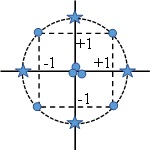
The response surface methodology is an effective statistical tool for experimental design, developing model, relationship between factors and research optimum condition16-19. The RSM main goals are to understand the position and topography of response surface including the minimum, maximum and ridge lines and find region where the important response occurs20. Two experimental designs are used in response surface methodology21, the Box-Behnken (BBD) and Central Composite Design (CCD). The CCD has three different design points: edge points as in two level designs ((1), star points at ((; (a( ≥ 1that take care of quadratic effects and center points. Three variants exist: circumscribed (CCC), inscribed (CCI) and face centered (CCF). The CCC design is the original central composite design that performs five-level testing. The edge points (factorial or fractional factorial points) are at the design limits. The star points are at some distance from the center depending on the number of factors in the design. The star points extend the range outside the low and high settings for all factors. The center points complete the design and verify the reproducibility. Figure 1 illustrates a CCC design. Completing an existing factorial or resolution V fractional factorial design with star and center points leads to this design. CCC designs provide high quality predictions over the entire design space, but care must be taken when deciding on the factor ranges. Especially, it must be sure that also the star points remain at feasible (reasonable) levels.
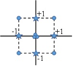
In CCI design, the star points are set at the design limits (hard limits) and the edge points are inside the range (Fig. 2). In a ways, a CCI design is a scaled down CCC design. It also results in five levels for each factor. CCI designs use only points within the factor ranges originally specified, so the prediction space is limited compared to the CCC design.

In CCF design the star points are at the center of each face of the factorial space, so α=(1 and only three levels are used (Fig. 3). Complementing an existing factorial or resolution V design with appropriate star points can also produce this design. CCF designs provide relatively high-quality predictions over the entire design range, but poor precision for estimating pure quadratic coefficients. They do not require using points outside the original factor range.
The experimental data are fitted by one of statistical model; Linear, Quadratic, Cubic or 2FI (two factor interaction). The linear coefficients for independent variables are A, B, and C, interactive term coefficient AB, AC and BC, quadratic term coefficient AA, BB and CC.
R2, R2Adj coefficient and adequate precision to check the model adequacies are:
where SCE: The sum of the squares of the residuals. SCT: The total sum of squares. (p-1) and (N-p) degrees of freedom. N: Number of experimental runs (excluding missing values). P: Number of terms in the model, including the constant. Conditions adequate model (probability value P < 0.05, lack of fit P > 0.05, R2, and R2Adj > 0.9). Adeq precision > 4. The analysis of variance ANOVA22 used to determine the differences between means.
2. Material and methods
2.1. Materials and sample preparations
Weight loss measurements were performed on the carbon steel XC38 samples with a rectangular form in perchloric acid medium with and without addition of different concentrations and size of polyvinylpyrrolidone. Carbon steel samples used as test materials contain: C: 0.37%, Mn: 0.68%, Cu: 0.16%, Cr: 0.077%, Ni: 0.059%, Si: 0.023%, S: 0.016%, Ti: 0.011%, Co: 0.009% and the balance being Fe. The samples were initially polished with emery paper starting with coarse until the mirror appearance was obtained, and were then washed with distilled water. They were cleaned again with acetone and, finally, dried using a hot air blower. Loss in weight of samples was resolved by finding the weight difference between the carbon steel substrates before and after immersion in corrosive attack. All measurements were done in triplicate, and the average value of the weight loss was noted. Each sample was weighed by an electronic balance ((0.0001g) and then placed in the acid solution (50 mL). The following equations were used to calculate the corrosion rate (CR) and the inhibition efficiencies (IE)23-25.
where (W is the weight loss (g); S is the total area of the specimen (cm2); t is the exposure time (h); CR and CRInh are the corrosion rates of carbon steel samples in the absence and presence of inhibitor, respectively (g cm-2h-1).
2.2. CCFCD Response surface design
In our study, the Central Composite Face-Centered Design (CCFCD) based on standard surface response methodology was used to obtain the individual and interactive effects of process parameters on inhibition efficiencies of PVP. Concentration (X1), Temperature (X2), Time of immersion (X3), different size of PVP (X4) and acid perchloric concentration (X5) were chosen as independent factors, while inhibition efficiencies (IE) was selected as response. Three levels (-1, 0, +1) for the variable range (see Table I) and five factors (see Table II below) were requiring 29 experimental runs.
Table I Levels of variables and factors considered for experimental design.
| Levels | ||||
|---|---|---|---|---|
| Variables | Factors | -1 | 0 | +1 |
| X1 | U1: Concentration (mol/L) | 5.0 10−5 | 2.52 10−3 | 5.0 10−3 |
| X2 | U2: Temperature (°C) | 20 | 40 | 60 |
| X3 | U3: Time of immersion (h) | 1 | 2 | 3 |
| X4 | U4: Different size (g/mol) | 8000 | 33000 | 58000 |
| X5 | U5: Acid concentration (mol/L) | 0.5 | 1 | 1.5 |
Table II Experimental Design Matrix of Inhibition Efficiency (Real values).
| Exp. N | X1 | X2 | X3 | X4 | X5 | IEObserved | IEPredicted |
|---|---|---|---|---|---|---|---|
| 1 | -1 | -1 | -1 | -1 | 1 | 31.35 | 31.33 |
| 2 | 1 | -1 | -1 | -1 | -1 | 74.67 | 74.73 |
| 3 | -1 | 1 | -1 | -1 | -1 | 11.75 | 11.88 |
| 4 | 1 | 1 | -1 | -1 | 1 | 48.19 | 48.06 |
| 5 | -1 | -1 | 1 | -1 | -1 | 36.37 | 36.53 |
| 6 | 1 | -1 | 1 | -1 | 1 | 58.63 | 58.52 |
| 7 | -1 | 1 | 1 | -1 | 1 | 05.98 | 05.95 |
| 8 | 1 | 1 | 1 | -1 | -1 | 54.76 | 54.80 |
| 9 | -1 | -1 | -1 | 1 | -1 | 62.50 | 62.67 |
| 10 | 1 | -1 | -1 | 1 | 1 | 70.49 | 70.39 |
| 11 | -1 | 1 | -1 | 1 | 1 | 14.89 | 14.87 |
| 12 | 1 | 1 | -1 | 1 | -1 | 73.17 | 73.22 |
| 13 | -1 | -1 | 1 | 1 | 1 | 47.31 | 47.32 |
| 14 | 1 | -1 | 1 | 1 | -1 | 90.05 | 90.13 |
| 15 | -1 | 1 | 1 | 1 | -1 | 25.45 | 25.61 |
| 16 | 1 | 1 | 1 | 1 | 1 | 56.41 | 56.30 |
| 17 | -1 | 0 | 0 | 0 | 0 | 29.24 | 28.65 |
| 18 | 1 | 0 | 0 | 0 | 0 | 64.68 | 64.89 |
| 19 | 0 | -1 | 0 | 0 | 0 | 82.18 | 81.92 |
| 20 | 0 | 1 | 0 | 0 | 0 | 59.42 | 59.31 |
| 21 | 0 | 0 | -1 | 0 | 0 | 59.57 | 59.40 |
| 22 | 0 | 0 | 1 | 0 | 0 | 58.12 | 57.91 |
| 23 | 0 | 0 | 0 | -1 | 0 | 62.27 | 62.15 |
| 24 | 0 | 0 | 0 | 1 | 0 | 77.25 | 76.99 |
| 25 | 0 | 0 | 0 | 0 | -1 | 69.51 | 68.63 |
| 26 | 0 | 0 | 0 | 0 | 1 | 56.03 | 56.53 |
| 27 | 0 | 0 | 0 | 0 | 0 | 64.65 | 65.14 |
| 28 | 0 | 0 | 0 | 0 | 0 | 64.63 | 31.33 |
| 29 | 0 | 0 | 0 | 0 | 0 | 64.64 | 74.73 |
The fit mode of inhibition efficiencies (IE) was modeled by a general function indicating the interaction between dependent and independent variables written as a second-degree polynomial equation,
where, X1, X2, X3, X4, and X5 are the input factors. a0 is the intercept; a1, a,2 a3, a4, and a5 are the linear coefficients. a11, a22, a33, a4, and a55 are the quadratic coefficients. a12, a13, a14, a15, a23, a24, a25, a34, a35 and a45 are the interaction coefficients.
3. Results and discussion
3.1. Validation and development of regression model
In the MODDE software, the residuals are plotted on a normal cumulative probability scale. This representation (Fig. 4) makes it possible to detect.
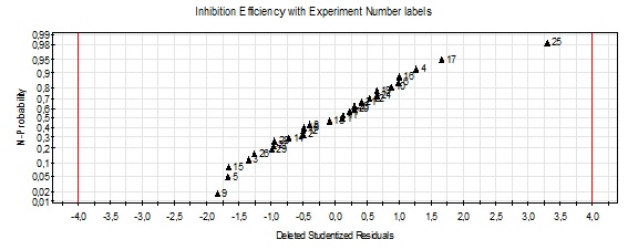
The normality of the residuals: when the residuals are normally distributed, the points describe a straight line, the aberrant values (atypical experiments): these are points of deviation from the line of normal probability, and having large absolute values of the studentized residuals26 standard deviation indicated by red lines in Fig. 1.
The value 4 is specified as the limit where the associated experience can be considered to be atypical. All experiences are not atypical experiments we can conclude that the residuals are normally distributed.
According to Fig. 2 analysis we can see that the experiments values are placed perfectly on the straight line indicated the perfect quality of the mathematical model.
3.2. Statistical results
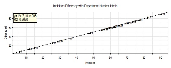
In this present work the observed Inhibition Efficiency for 29 experimental runs are presented in Table II. The data of Table V are used to determine the coefficient of the polynomial equation (see Sec. 2.2) and optimum parameter’s that influenced the efficiency of polymer network. The estimated coefficients are shown in Table V.
Table III Statistical results of experimental design model.
| R2 | R2Adj | Q2 | SDY | RSD | N | Model Validity | Reproducibility |
|---|---|---|---|---|---|---|---|
| 0.999797 | 0.99929 | 0.988461 | 21.2081 | 0.565237 | 29 | -0.2 | 1 |
| DF=8 | Conf. lev. =0.95 | Cond. No =7.2 |
Table IV The analysis of variance for the quadratic model of inhibition efficiency.
| Inhibition Efficiency | DF | SS | MS (variance) | F | p | SD |
|---|---|---|---|---|---|---|
| Total | 29 | 98041.5 | 3380.74 | |||
| Constant | 1 | 85447.6 | 85447.6 | |||
| Total Corrected | 28 | 12593.9 | 449.784 | 21.2081 | ||
| Regression | 20 | 1288.1 | 629.407 | 1857.65 | 0.000 | 25.088 |
| Residual | 8 | 2.55594 | 0.319493 | 0.565237 | ||
| Lack of Fit | 6 | 2.55574 | 0.425957 | 4256.94 | 0.000 | 0.652654 |
| (Model Error) | ||||||
| Pure Error | 2 | 2.00124 10−4 | 1.00062 10−4 | 1.00031 10−2 | ||
| Conf. lev. =0.95 |
Table V Estimated regression coefficients of factors, interaction and P-values of the model.
| Inhibition Efficiency | Coeff. SC | P |
|---|---|---|
| Constant | a0 = 65.1385 | 4.92993 e−18 |
| Con | a1 = 18.1228 | 9.53897 e−15 |
| Temp | a2 = -11.3072 | 4.14372 e−13 |
| Tim | a3 = -0.749996 | 0. 000493058 |
| Siz | a4 = 7.41944 | 1.19943 e−11 |
| Aci | a5 = -6.05278 | 6,08538−11 |
| Con*Con | a11 = -18.3618 | 2.46261 e−11 |
| Temp*Temp | a22 = 5.47461 | 3.53143 e−7 |
| Tim*Tim | a33 = -6.4804 | 9.48598 e−8 |
| Siz*Siz | a44 = 4.4346 | 1.78911 e−6 |
| Aci*Aci | a55 = -2.55539 | 0. 000103947 |
| Con*Temp | a12 = 3.63437 | 5,60208 e−9 |
| Con*Tim | a13 = -0.0806205 | 0. 583986 not significant |
| Con*Siz | a14 = -0.676875 | 0. 00137294 not significant |
| Con*Aci | a15 = -1.39937 | 9.12921 e−6 |
| Temp*Tim | a23 = 0.0781245 | 0. 595464 not significant |
| Temp*Siz | a24 = -1.25563 | 2,03556 e−5 |
| Temp*Aci | a25 = 1.00937 | 9. 77612 e−5 |
| Tim*Siz | a34 = 0.524378 | 0.00594903 not significant |
| Tim*Aci | a35 = 1.17938 | 3.21538 e−5 |
| Siz*Aci | a45 = -1.79187 | 1.40663 e−6 |
The statistical analysis calculation was assured by analysis variance (ANOVA) given in Table III. The adequacy of the model and the determination of R2 coefficient indicated good model. Ghasemzadeh et al.,27 found that ANOVA for predicted model of antioxidant activity was significant (F - value17.21, P < 0.0001) with a good coefficient of determination (R2 = 0.98). In addition, R2 calculation indicates a good correlation between experiments and predicts data (using MODDE Software Version 9.1)28.
The methods to estimate the model coefficients are Partial Least Squares (PLS)29,30 and Multiple Linear Regression (MLR)31. In our study, the MLR method was used for the estimation of model coefficients.
The determination coefficients R2, R2Adj and Q2 are the statistical results of experimental design model presented; first R2 (see Eq. (2) and Table III) for evaluated the correlation between two data predicted and measured experiments, the second coefficient R2Adj (see Eq. (3) and Table III) is also used to measure the quality of fit, the Q2 coefficient shows an estimate of the future prediction precisions, their values should be greater than 0.1 for a significant model and greater than 0.5 for a good model. The Table III shows the values of R2, R2Adj and Q2.
Where SDY represents the Standard Deviation of the Y (response) and RSD corresponds to the Residual Standard Deviation.
Analyses of Table III revealed R2 value of 0.99, indicated that the model can explain 99% of the data variation and 1% not explained. Chauhan and Gudta32 emphazed in their work on the acceptance of any model with R2 > 0.75, but according to Koocheki et al. postulated that a large value of R2 does not always imply that the regression model is good, it is necessary to check at the same time the value of R2Adj. Differently the model is adequate for prediction in the range of experimental variables. The value R2 of 0.999797 and R2Adj of 0.99929 consequently confirmed that the model was highly significant, which designated a good agreement between predicted and experimental inhibition efficiency in PVP polymer network. In study of Rai et al.34 R2 and R2Adj should be within 20% to be in good agreement. Reproducibility is the variation of replicates compared to overall variability here a value 1 > 0.5 is warranted. The validity of model is -0.2 < 0.25 indicates statistically significant model problems. The model validity might be low in very good models (Q2 > 0.9) due to high sensitivity in the test or extremely good replicates35. The analysis of variance ANOVA of each term of quadratic model is tabulated in Table IV. Analyzes were performed using Fisher’s “F” test. According to Rene et al.36, the “F” value with a low probability “P” value generally indicates high significance of the regression model. Based on the ANOVA summary (Table IV), the model was found to be statistically significant (P < 0.05) at the 95% confidence level. Due to the lower value for lack of fit and the lower “P” value (P = 0), the effects are highly significant.
3.3. Regression coefficients and probability
The linear, quadratic and interaction coefficients of different factors effects 𝑎 0 is constant; a1 (Concentration), a2 (Temperature), a3 (Time), a4 (different size) and a5 (Acid concentration) a11, a22, a33, a44, a55, a12, a13, a14, a15, a23, a24, a25, a34, a35, and a45 obtained from the experimental design model are represented in Table V.
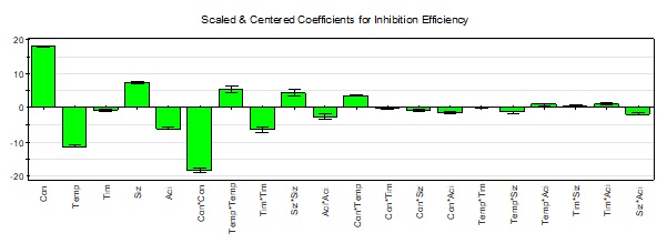
In the first column, analysis of the coefficients indicated that only four were not significant a13 (Concentration*Time), a13 (Concentration*Size), a23 (Temperature*Time) and a34 (Time*Size), while the other factors are all significant (P < 0.0001). However the positive and negative signs in the model signify a synergetic and antagonistic effect respectively. Furthermore, Inhibition Efficiency increases with concentration and size of PVP and decrease with temperature and acid concentration37.
The histograms of the coefficient’s effects on the inhibition efficiencies (IE) of PVP are shown in Fig. 6. We note that the most influential factor is a1 = 18.12 (Concentration) flowed by a2 = -11.31 (Temperature), a4 = 7.42 (different size) and a5 = -6.05 (Acid concentration). The coefficient a3 = -0.75 (Time) is considered negligible compared to the other variables. We can say that the concentration, temperature and different size of PVP compared to immersion time, are the most influential factors on inhibition efficiencies (IE). Moreover, the positive coefficients for the independent variables indicated a favorable effect on the mechanical properties38. The pure quadratic effect a11 (Concentration*Concentration) is the most influential and greater than that linear effect a1. It is important to note that the Eq. (8) is only valid in the range 5.010-5 < Concentration (mol/L) < 5.010-3, 20 < Temperature (°C) < 60, 1 < Time (hrs) < 3h, 8000 < Different size of PVP (g/mol) < 58000 and 0.5 < perchloric Acid Concentration (mol/L) < 1.5.
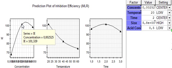
Prediction plot Wizard allowed us to vary each variable independently of the others. The prediction plots of inhibition efficiency in PVP polymer by MLR methodology shows that the (IE) maximum of 101.329% is obtained for concentration of 2.5 (mol/L), temperature around 20 °C, immersion time of 2 hours, PVP size of 58000 (g/mol) and perchloric acid concentration of 0.5 (mol/L) (Fig. 7).
4. Analysis of response surfaces and optimization conditions
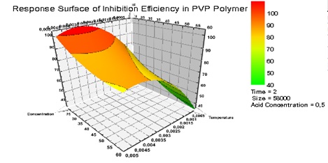
The optimum condition of each factor to have maximum value of inhibition efficiencies (IE) must be assured by three-dimensional response surfaces plot and their projections. From the results obtained from the inhibition efficiency prediction plots (Fig. 7). Figure 8 represents the response surface illustrating the optimum of inhibition efficiency (IE) at two hours, different size 58000 (g/mol) and acid concentration of 0.5 (mol/L).
To confirm our results of prediction plot wizard, we exploit all the 4D contour plots to find the best optimum. We fixed the size of the PVP at 58000 (g/mol) by varying each time the other parameters from the low level to the high level. Figures 6 illustrate the 4D contour curves of inhibition efficiency (IE). Figure 9a) illustrates the 4D contour for the value of acid concentration at the maximum value (1.5 mol/L), Fig. 9b) that in the center of domain (1 mol/L) and Fig. 9c). corresponds to the minimum value (0.5 mol/L).
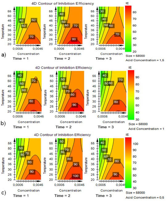
Figure 9 a) 4D Contour Plot of Inhibition Efficiencies (IE) for a PVP Size of 58000g/mol vs reaction Concentration, Temperature, Time, and Acid Concentration (High). b) 4D Contour Plot of Inhibition Efficiencies (IE) for a PVP Size of 58000 g/mol vs reaction Concentration, Temperature, Time, and Acid Concentration (Center). c) 4D Contour Plot of Inhibition Efficiencies (IE) for a PVP Size of 58000 g/mol vs reaction Concentration, Temperature, Time, and Acid Concentration (Low).
The results obtained show that the optimum is reached at a temperature of 20 °C, the immersion time of 2 h, the concentration of 0.0025 (mol/L) and an acidity of 0.5 (mol/L) using the size of the PVP of 58000 (g/mol).
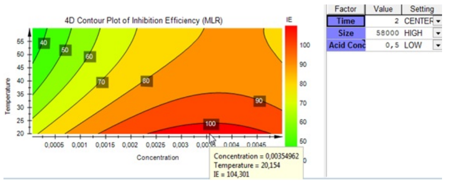
To better observe the optimum, we fixed the immersion time at 2 h, the size of the PVP at 58000 (g/mol), the acid concentration at 0.5 (mol/L). Figure 10 illustrates the 4D contour plot using the MLR method. The optimum of (IE) obtained is 104.301% for a concentration of 0.00354962 (mol/L) and a temperature of 20.154 °C. This study clearly shows that these results are in good agreement with those obtained experimentally.
5. Conclusion
The effect of five independent factors as Concentration, Temperature, Time of immersion, Different size of PVP and Acid perchloric concentration on the inhibition efficiencies (IE) in PVP polymer was investigated in this paper, using the Central Composite Face-Centered Design CCFCD, quadratic model of response surface methodology (RSM) applying Multiple Linear Regression (MLR) fit. A linear, quadratic and interaction model terms were developed. Only, the interaction effects of Con*Tim, Con*Siz, Temp*Tim and Tim*Siz were negligible while the other coefficients are significant. The correlation coefficient R2 of 0.99 indicated a good agreement between the experimental and predicts value. RSM was effectively applied to determine the optimal condition for the maximum (IE) which is 104.301% corresponded to the optimum factors: Concentration of 3.55 10-3 mol/L, Temperature of 20.154 °C, Immersion time of 2 h, PVP size of 58000 g/mol and perchloric acid Concentration of 0.5 mol/L. From this study, we can say that the experiments design methodology using response surface could be generally used in professional industry and chemistry. Particularly, it is approached in polymer domain for inhibition efficiencies (IE) modeling.

