SciELO - Scientific Electronic Library Online

 
vol.66 número3Fractal model equation for spontaneous imbibitionNew analytical solutions of fractional symmetric regularized-long-wave equation índice de autoresíndice de materiabúsqueda de artículos
Home Pagelista alfabética de revistas  

Servicios Personalizados

Revista

Articulo

Indicadores

Links relacionados

  • No hay artículos similaresSimilares en SciELO

Compartir


Revista mexicana de física

versión impresa ISSN 0035-001X

Rev. mex. fis. vol.66 no.3 México may./jun. 2020  Epub 26-Mar-2021

https://doi.org/10.31349/revmexfis.66.291 

Research

Gravitation, Mathematical Physics and Field Theory

Highly dispersive optical solitons having Kerr law of refractive index with Laplace-Adomian decomposition

O. González-Gaxiolaa  * 

Anjan Biswasb  c  d  e 

Ali Saleh Alshomranic 

aDepartamento de Matemáticas Aplicadas y Sistemas, Universidad Autónoma Metropolitana-Cuajimalpa. Vasco de Quiroga 4871, 05348 Mexico City, Mexico.

bDepartment of Physics, Chemistry and Mathematics, Alabama A&M University, Normal, AL 35762-7500, USA.

cDepartment of Mathematics, King Abdulaziz University, Jeddah-21589, Saudi Arabia.

dDepartment of Applied Mathematics, National Research Nuclear University, 31 Kashirskoe Shosse, Moscow-115409, Russian Federation.

eDepartment of Mathematics and Statistics, Tshwane University of Technology, Pretoria-0008, South Africa.


Abstract

This paper studies highly dispersive optical solitons, having Kerr law of refractive index, numerically. The adopted scheme is Laplace-Adomian decomposition method. Bright soliton solutions are displayed along with their respective error analysis.

Keywords: Nonlinear Schrödinger equation; bright solitons; higher-order dispersion; Laplace-adomian decomposition method

PACS: 02.30.Jr; 02.30.Uu; 02.60.Cb; 44.05.+e

1. Introduction

The concept of highly dispersive optical solitons emerged during 2019 as an extension and/or generalization to cubic-quartic solitons. Analytical results are abundant and stem from this concept, and these have been recovered after implementing of algorithms. These include extended trial function method, F-expansion scheme, Jacobi’s elliptic function expansion, exp-expansion and others [1-5]. The conservation laws for such solitons have also been reported [3]. Therefore, it is now time to turn the page and explore this topic from a numerical perspective. This paper, therefore. addressed highly dispersive optical solitons, having Kerr law of refractive index, by the aid of the Laplace-Adomian decomposition scheme. The focus on this paper will be on bright optical solitons. The scheme is first explicitly elaborated and subsequently implemented into the model equation successfully. The details are sketched in the rest of the paper.

2. Governing equation

The dimensionless form of NLSE with Kerr law nonlinearity in presence of dispersion terms of all orders is [6]:

iqt+ia1qx+a2qxx+ia3qxxx+a4qxxxx+ia5qxxxxx+a6qxxxxxx+bq2q=0, (1)

where q = q(x,t) is a complex-valued function of x (space) and t (time) and i = √-1 The first term represents linear temporal evolution. The next six terms are dispersion terms that make the solitons highly dispersive. These are given by the coefficients of a K for 1 ≤ k ≤ 6, which are intermodal dispersion (IMD), group velocity dispersion (GVD), third-order dispersion (3OD), fourth-order dispersion (4OD), fifth-order dispersion (5OD) and sixth-order dispersion (6OD) respectively. Finally, b indicates the coefficient of self-phase modulation based on cubic or Kerr nonlinearity.

2.1. Bright solitons

The bright 1-soliton solution to (1) was recently found by the authors in [6,7] using the semi-variational principle and is given by

qx, t=AsechBx-νt+sech3Bx-νtei-κx+ωt+θ0 (2)

In Eq. (2), v is the soliton velocity, ω is the angular velocity, κ is the soliton frequency, and θ 0 is the phase center.

In [7], the amplitude A of the 1-soliton was calculated as:

A= -182.946a6B6-16.874P3B4+11.847P2B226.118b12 (3)

where:

P1=ω+a1κ-a2κ2-a3κ3+a4κ4+a5κ5-a6κ6 (4)

P2=a2+3a3κ-6a4κ2-10a5κ3+15a6κ4 (5)

P3= a4+5a5κ-15a6κ2 (6)

Besides, the inverse width B of the 1-soliton is a real root of the equation:

670.813a6B6-59.059P3B4+35.541P2B2-99.33P1=0. (7)

The velocity v is given by

ν=a1-2a2κ-3a3κ2+5a5κ4-6a6κ5. (8)

Finally, there are the following two relationships between the soliton frequency κ and some of the coefficients of Eq. (1), these are given by

a3-4a4κ-10a5κ2+20a6κ3=0anda5-6a6κ=0.

3. Method applied

In this section, we will describe the basic theory and algorithm of the Laplace-Adomian decomposition method (LADM), used to solve nonlinear partial differential equations, and that was first proposed in [9,10].

Let us look for soliton solutions of Eq. (1) in the form q(x, t) = u(x, t) + iv(x, t). Then we can decompose the Eq. (1) in its real and imaginary parts, respectively as

ut=-a1ux-a2uxx-a3uxxx-a4uxxxx-a5uxxxxx-a6uxxxxxx-buu2+v2 (9)

vt= -a1vx+a2vxx-a3vxxx+a4vxxxx-a5uxxxxx+a6vxxxxx+buu2+v2 (10)

To give analytical approximate solutions for Eq. (1) using LADM, we first rewrite the Eqs. (9) and (10) in the following operator form

Dtu=-a1Dx1v-a2Dx2u-a3Dx3v-a4Dx4u-a5Dx5v-a6Dx6u+N1u, v (11)

Dtu=-a1Dx1v+a2Dx2u-a3Dx3v+a4Dx4u-a5Dx5v+a6Dx6u+N2u, v (12)

with initial conditions u(x, 0) = ℜ(q(x, 0)) and v(x, 0) = ℑm(q(x, 0)).

In the equations system (11)-(12), the operator D t denotes derivative with respect to t, whereas that D j x is the j-th order linear differential operator δ j /δ j , and N κ represents nonlinear differential operators for k = 1, 2.

The method consists of first applying the Laplace transform ℒ to both sides of equations in system (11)-(12) and then, by using initial conditions, we have

ux, s=ux, 0s+1sL-a1Dx1u-a2Dx2v-a3Dx3u-a4Dx4v-a5Dx5u-a6Dx6v+N1u,v (13)

vx,s= vx, 0s+1sL-a1Dx1v+a2Dx2u-a3Dx3v+a4Dx4u-a5Dx5v+a6Dx6u+N2u,v (14)

Thus, by applying the inverse Laplace transform ℒ-1, we obtain

ux, t=ux, 0+L-11sL-a1Dx1u-a2Dx2v-a3Dx3u-a4Dx4v-a5Dx5u-a6Dx6v+N1u,v (15)

vx, t=vx, 0+L-11sL-a1Dx1v-a2Dx2u-a3Dx3v-a4Dx4u-a5Dx5v-a6Dx6u+N2u,v (16)

According to the standard Adomian decomposition method, the solutions u and v can be expressed in an infinite series as follows

u(x,t)=n=0un(x,t),v(x,t)=n=0vn(x,t) (17)

Also, the nonlinear terms can be written as

N1u,v=-bvu2+v3=-bn=0Bnu0, u1, ,un; v0, v1, , vn (18)

and

N2u,v=-buv2+u3=bn=0Bnu0, u1, ,un; v0, v1, , vn (19)

where A n and B n are the Adomian?s polynomials [11,12], which are defined by

Anu0,, un;v0,,vn=1n!dndλn×N1i=1λiui;i=1λiviλ=0n=0, 1, 2, (20)

Bnu0,, un;v0,,vn=1n!dndλn× N2i=1λiui;i=1λiviλ=0n=0, 1, 2, (21)

On making the substitution of Eqs. (17) and (18) into Eqs. (15) and (16), we can arrive at

n=0un=u(x,0)+L-1[1sL{-(a1Dx1+a3Dx3+a3Dx5)n=0un-(a2Dx2+a4Dx4+a6Dx6)n=0vn-bn=0An}] (22)

n=0vn=v(x,0)+L-1[1sL{-(a1Dx1+a3Dx3+a3Dx5)n=0vn+(a2Dx2+a4Dx4+a6Dx6)n=0un+bn=0Bn}] (23)

Now, according to LADM, The following recursive schemes can be constructed

u0(x,t)=Re(q(x,0)),un+1(x,t)=L-1[1sL{-(a1Dx1+a3Dx3+a3Dx5)un-(a2Dx2+a4Dx4+a6Dx6)vn-bAn}],n0, (24)

v0(x,t)=Im(q(x,0)),un+1(x,t)=L-1[1sL{-(a1Dx1+a3Dx3+a3Dx5)vn+(a2Dx2+a4Dx4+a6Dx6)un+bBn}],n0. (25)

Being N1(u, v) = vu2 + v3 and N2(u, v) = uv2 + u3, using the formulas (20) and (21) some terms of Adomian’s polynomials An and Bn are given by

A0=u02v0+v03,A1=2u0u1v0+u12v0+3v02v1,A2=2u0u2v0+u12v0+2u0u2v1+u12v1+3v02v2+3v0v12,A3=2u0u3v0+2u1u2v0+2u0u2v1+u12v1+2u0u1v2+u02v3+3u02v3+6u0v1v2+u13A4=v0u22+2u0v0u4+2v0u1u3+2u0v1u3+2u1v1u2+2u0v2u2+u12v2+2u0v1u3+u02v4+3v02v4+6v0v1v3+3v0v22+3v12v2 (26)

and

B0=v02u0+u03,B1=2v0v1u0+v12u1+3u02u1,B2=2v0v2u0+v12u0+2v0v2u1+v12u2+3u02u2+3u0u12,B3=2v0v3u0+2v1v2u0+2v0v2u1+v12u1+2v0v1u2+v02u3+3u02u3+6u0u1u2+u13B4=u0v22+2v0u0v4+2u0v1v3+2v0u1v3+2v1u1v2+2v0u2v2+v12u2+2v0u1v3+v02u4+3u02u4+6u0u1u3+3u0u22+3u12u2 (27)

Finally, in conjunction with Eq. (24) and Eq. (25), all components of u(x, t) in Eq. (17) will be easily determined; therefore, the complete solution u(x, t) in Eq. (17) can be formally established. LADM provides a reliable technique that requires less work if compared with traditional techniques.

4. Numerical simulations

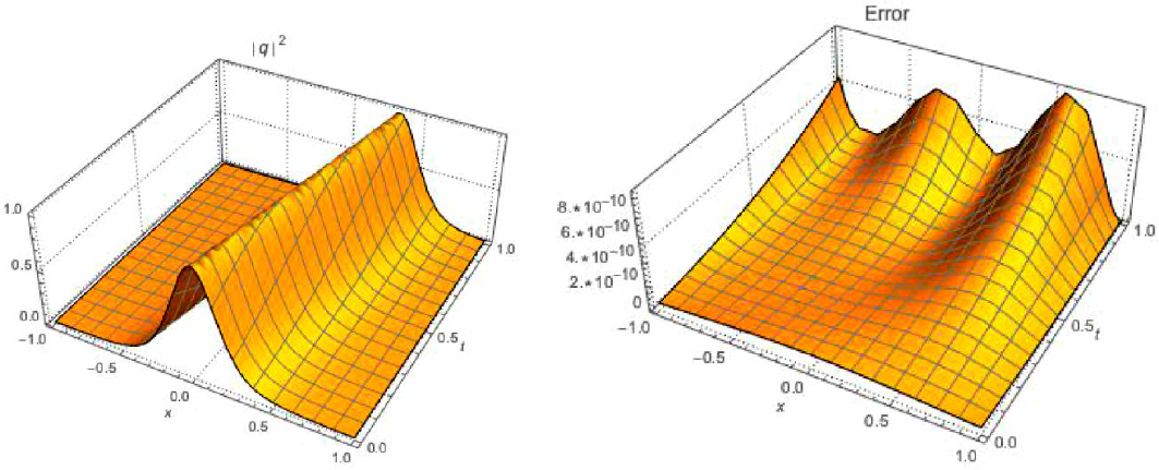
To illustrate the ability, reliability, and accuracy of the proposed method to find solutions of Eq. (1) in the case of bright solitons, some examples are provided. The results reveal that the method is very effective and simple. We now consider the initial condition at t = 0 from Eq. (2)

qx,0=AsechBx+sech3Bxei-κx+θ0 (28)

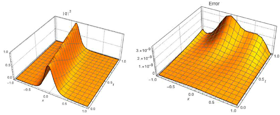
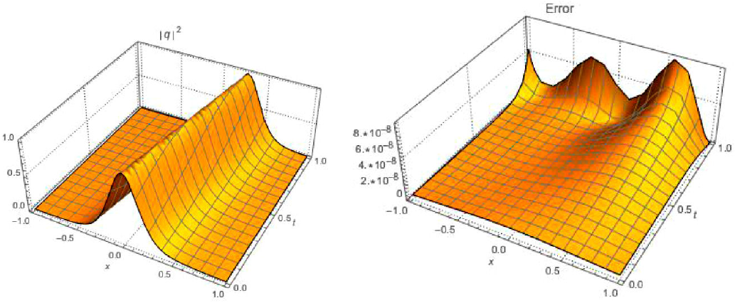
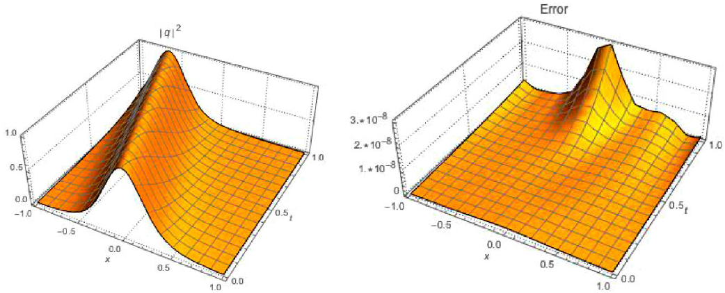
We now perform the simulation of the four cases listed in Table I, and the results and the respective absolute errors are shown in Figs. 1, 2, 3, and 4.

Table I Coefficients of Eq. (1) for bright solitons. 

Cases a1 a2 a3 a4 a5 a6 b κ ω θ0 ν N |Max Error|
1 1.2 0.01 0.024 0.50 4.20 0.33 −1.20 0.01 0.3 1.2 1.19 15 8.0 × 10⁻¹⁰
2 1.5 0.07 0.058 0.25 3.20 0.16 −1.10 0.03 0.1 1.4 1.49 15 3.0 × 10⁻⁹
3 1.0 0.09 0.013 0.12 1.00 0.08 −1.00 −0.02 0.7 1.6 1.00 12 8.0 × 10⁻⁸
4 1.6 0.04 −0.030 0.80 1.20 0.10 −1.30 −0.01 0.3 1.3 1.60 12 3.0 × 10⁻⁸

Figure 1 Case 1: Numerically computed profile (left) and absolute error (right). 

Figure 2 Case 2: Numerically computed profile (left) and absolute error (right). 

Figure 3 Case 3: Numerically computed profile (left) and absolute error (right). 

Figure 4 Case 4: Numerically computed profile (left) and absolute error (right). 

5. Conclusions

This paper addressed highly dispersive optical solitons, with Kerr law nonlinearity, by the aid of the Laplace-Adomian decomposition scheme. The focus was on bright solitons. The numerical results supplemented the analytical results, there were reported earlier, and the agreement is to a T. The error analysis was also profoundly impressive, as well. This shows extreme promise of the numerical algorithm that has been implemented in this paper. Thus, the results of this paper will be extended to additional laws of the nonlinear refractive index. These are cubic-quartic law, polynomial law, nonlocal nonlinearity, and others. Additionally, the results will be extended to birefringent fibers. The results of such research activities are on the horizon and are soon going to be made visible.

Acknowledgments

This project was funded by the Deanship of Scientific Research (DSR), King Abdulaziz University, Jeddah, Saudi Arabia under grant no. (KEP-15-130-40). The authors, therefore, acknowledge with thanks to DSR technical and financial support.

References

1. N. A. Kudryashov, Construction of nonlinear differential equations for description of propagation pulses in optical fiber, Optik 192 (2019) 162964, https://doi.org/10.1016/j.ijleo.2019.162964. [ Links ]

2. N. A. Kudryashov, Solitary and periodic waves of the hierarchi for propagation pulse in optical fiber, Optik 194 (2019) 163060, https://doi.org/10.1016/j.ijleo.2019.163060. [ Links ]

3. A. Biswas, A. H. Kara, A. S. Alshomrani, M. Ekici, Q. Zhou, and M. R. Belic, Conservation laws for highly dispersive optical solitons, Optik 199 (2019) 163283, https://doi.org/10.1016/j.ijleo.2019.163283. [ Links ]

4. H. U. Rehman, N. Ullah, and M. A. Imran, Highly dispersive optical solitons using Kudryashov’s method, Optik 199 (2019) 163349, https://doi.org/10.1016/j.ijleo.2019.163349. [ Links ]

5. O. Pavón-Torres, M. A. Agüero, T. L. Belyaeva, A. Ramirez, and V. N. Serkin, Unusual self-spreading or self-compression of the cubic-quintic NLSE solitons owing to amplification or absorption, Optik 184 (2019) 446, https://doi.org/10.1016/j.ijleo.2019.04.103. [ Links ]

6. A. Biswas, M. Ekici, A. Sonmezoglu, and M. R. Belic, Highly dispersive optical solitons with Kerr law nonlinearity by F-expansion, Optik 181 (2019) 1028, https://doi.org/10.1016/j.ijleo.2018.12.164. [ Links ]

7. R. W. Kohl, A. Biswas, M. Ekici, Q. Zhou, S. Khan, A. S. Alshomrani, and M. R. Belic, Highly dispersive optical soliton perturbation with Kerr law by semi-inverse variational principle, Optik 199 (2019) 163226, https://doi.org/10.1016/j.ijleo.2019.163226. [ Links ]

8. A. Biswas, M. Ekici, A. Sonmezoglu, M. R. Belic, Highly dispersive optical solitons with Kerr law nonlinearity by extended Jacobi’s elliptic function expansion, Optik 183 (2019) 395, https://doi.org/10.1016/j.ijleo.2019.02.050. [ Links ]

9. G. Adomian, Solving Frontier Problems of Physics: The Decomposition Method (Springer, Dordrecht, 1994), https://doi.org/10.1007/978-94-015-8289-6. [ Links ]

10. S. A. Khuri, A Laplace decomposition algorithm applied to a class of nonlinear differential equations, J. Appl. Math. 1 (2001) 141, https://doi.org/10.1155/S1110757X01000183. [ Links ]

11. R. Rach, A convenient computational form for the Adomian polynomials, J. Math. Anal. Appl. 102 (1984) 415, https://doi.org/10.1016/0022-247X(84)90181-1. [ Links ]

12. A.-M. Wazwaz, A new algorithm for calculating adomian polynomials for nonlinear operators, Appl. Math. Comput. 111 (2000) 33, https://doi.org/10.1016/S0096-3003(99)00063-6. [ Links ]

Received: November 05, 2019; Accepted: December 16, 2019

Creative Commons License This is an open-access article distributed under the terms of the Creative Commons Attribution License