Numerical experiments on geostrophic adjustment

 

A. WIIN-NIELSEN

The Collstrup Foundation, Royal Danish Academy of Sciences and Letters, H.C. Andersens Blvd. 37, 1553 Copenhagen V, Denmark

 

(Manuscript received, August 18, 2000; accepted in final form June 4, 2001)

 

RESUMEN

El problema bien conocido del ajuste geostrófico ha sido reinvestigado empleando primero un modelo de una atmósfera horizontal con una superficie libre. Las ecuaciones básicas en este modelo son las dos ecuaciones de movimiento para las componentes de velocidad modificadas para contener solamente las variaciones este-oeste y la ecuación de continuidad manejada de la misma manera. Un término friccional lineal se incluye en las ecuaciones y el forzamiento del modelo atmosférico está incluido en la ecuación de continuidad.

El caso zonal se describe en las secciones 2 y 3. Las ecuaciones son integradas numéricamente a partir de un estado de reposo y una superficie superior horizontal. Si se obtuviese el ajuste geostrófico las componentes zonales de la velocidad deberían ser pequeñas, mientras que las componentes de velocidad meridionales deberán estar en equilibrio aproximado con la componente geostrófica calculada a partir del gradiente zonal geopotencial.

Se encuentra por integración de las ecuaciones durante 20 días que los requisitos son satisfechos. La integración numérica del conjunto de las ecuaciones primitivas se llevan a cabo en el espacio de onda numérico, pero los resultados se presentan como variaciones continuas en las direcciones oeste-este. Se muestra que los ajustes geostróficos se alcanzan después de un par de días.

El estado final del proceso de ajuste se obtiene empleando varias especificaciones del forzamiento. En tanto que los estados finales naturales son diferentes, el ajuste geostrófico se encuentra en cada caso. Un caso basado en la serie de Fourier completa se incluye también en la Sección 3.

El problema de ajuste se trata también en el caso meridional en las secciones 4 y 5 usando la misma estrategia como se describe arriba. La Sección 6 contiene una solución del problema de ajuste empleando un modelo de ecuaciones primitivas de dos niveles sosteniéndose solamente las variaciones en la dirección zonal.

 

ABSTRACT

The well known geostrophic adjustment problem has been reinvestigated using first a model of a homogeneous atmosphere with a free surface. The basic equations in this model are the two equations of motion for the horizontal velocity components modified to contain only the east-west variations and the continuity equation treated in the same way. A linear frictional term is included in the equations, and the forcing of the model atmosphere is included in the continuity equation.

The zonal case is described in Sections 2 and 3. The equations are integrated numerically from an initial state of rest and a horizontal upper surface. If geostrophic adjustment should be obtained, the zonal velocity components should be small, while the meridional velocity components should be in approximate balance with the geostrophic component computed from the zonal geopotential gradient.

It is found by integrating the equations for 20 days that the above requirements are satisfied. The numerical integrations of the set of primitive equations are carried out in wave number space, but the results are presented as continuous variations in the west-east directions. It is shown that geostrophic adjustment is reach after a couple of days.

The final state of the adjustment process is obtained using several specifications of the forcing. While the final states naturally are different, the geostrophic adjustment is found in each case. A case based on full Fourier series is also included in Section 3.

The adjustment problem is also treated in the meridional case in section 4 and 5 using the same strategy as described above.

Section 6 contains a solution of the adjustment problem using a two-level, primitive equation model maintaining only the variations in the zonal direction.

Key words: geostrophy, adjustment, geostrophic adjustment.

 

1. Introduction

The observed large-scale atmospheric winds are quasi-geostrophic. It has been attempted to explain this fact by investigations of processes leading to geostrophic winds. These processes are normally classified under the name of "geostrophic adjustment". The first attempt to solve the problem was made by Rossby (1937, 1938). The same problem was treated in more detail by Cahn (1945). Later investigations were carried out by Obukhov (1949), Bolin (1953), Kibel (1955) and Blumen (1972). The first investigations considered quite simple systems. We may describe the main aspects of the problem by considering at the initial time a constant zonal velocity bounded by walls at given latitudes to the north and the south. The effect of the Coriolis force is to create a height difference between the southern and the northern boundaries. The final state is a geostrophic equilibrium. Initially all the energy is in the form of kinetic energy, but part of the kinetic energy is converted to potential energy during the adjustment to a geostrophic state. A penetrating analysis of the classical adjustment problem has been carried out by Kuo (1998). He started from linear equations and neglected forcing and dissipation.

The same problem was treated by Winninghoff (1968). He used numerical integrations to obtain the solutions, but the initial conditions were still quite simple, and no forcing and dissipation were introduced in the equations.

Problems of this kind contain some simplifying aspects, because the initial state is rather artificial. The adjustment process as described by the various models disregards all references to the heating of the atmosphere and the dissipation of the kinetic energy.

One may of course also say that the results of long integrations of the equations for a general circulation model starting from a state of rest and giving a good simulation of the observed atmospheric state is a verification of a geostrophic adjustment.

The purpose of the present paper is to use mainly a quite simple model of a homogeneous fluid with a free surface based on the equations of motion for the two horizontal wind components and on the continuity equation. The heating of the atmosphere is in the first two models simulated by a forcing function in the continuity equation as discussed by Wiin-Nielsen (1999). Due to the forcing it is required to add frictional terms in the equations of motion. All experiments start from a state of rest.

It is the purpose to show that numerical integrations of these simple models will lead to geostrophic adjustment.

A two-level primitive equation model with variations in the zonal direction only is also used to illustrate the adjustment process. In this case we include a heating in the thermodynamic equation and frictional terms in the two equations of motion.

 

2. The model equations in the zonal case

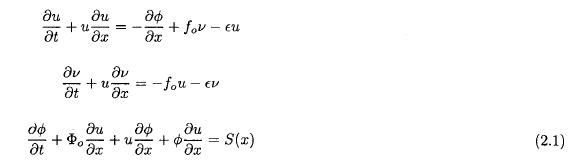
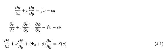
The model equations are formulated in one space dimension - in this case the x-direction - and in time. They have to contain the Coriolis force. The Coriolis parameter may be considered as constant since we use only the east-west direction in the model. The forcing is denoted by S(x). We include the advection terms in the x-direction in the two equations of motion as well as the advection and the divergence term in the continuity equation. The model equations are as given in (2.1).

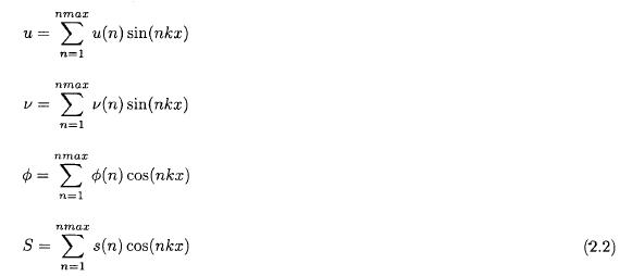
S is the amount of fluid added or subtracted in such a way that the net addition vanishes, e is the frictional coefficient, and f_o is a standard value of the Coriolis parameter. The equations in (2.1) are transformed to wave number space. It is a simplification to assume that the forcing and the geopotential are cosine-series, while the two velocity components are sine-series as given in (2.2). It is also possible to include both of the trigonometric functions in each of the series, but it gives twice as many equations and additional sums to evaluate. The main results can, however, be obtained with the simple model.

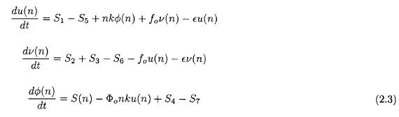
The three spectral equations may be written as seen in (2.3).

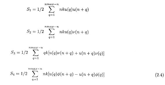
The three basic equations for the system contain seven sums. They are defined in (2.4) and (2.5).

An experiment starts from a defined forcing (S(x)) which is constant during the integration. As a first step the Fourier components of the forcing, i.e. S(n), are computed for all n. The initial state has u(n) = v(n) = j(n) = 0 for all the permitted values of n. In the integrations we have used Φ₀ = g₀² = 1.0 x 10⁵ m² s^-2, e = 4.0 X 10^-6 s^-1, and L = 28000 km, corresponding to the length of a latitude circle at 45 degrees of latitude. The numerical integrations have been carried out using Heun's numerical scheme with a time step of a few minites and with n_max =20. To test the accuracy some integrations were carried out with larger values of the maximum wave number, but the chosen value is sufficient for accuracy in the results. The integrations have been carried out for 480 hours, equal to 20 days, to ensure that the model has arrived at a steady state. As a final step in the program the spectral values have been converted into functions of x, the nondimensional value of the independent variable equal to the dimensional length divided by L.

 

3. The results of the zonal experiments

In the first experiment it is assumed that the forcing is positive and constant in the interval [0.25, 0.75] and negative and constant for the remaining part of the interval from 0 to 1. The constant values of S(x) in the three intervals are selected in such a way that the net forcing over the whole interval is zero. The components, S(n), of this idealized distribution are computed.

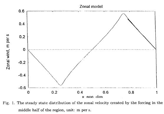
Since we add fluid in the central part of the interval and remove fluid in the other parts, one would expect that fluid will be moved away from the centre in both directions.

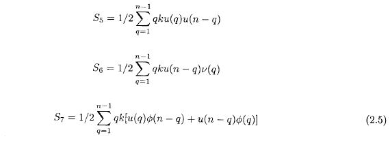
Figure 1 shows the steady state solution for the zonal wind component, u = u(x), calculated from u(n) after the integration of the model for 20 days. As expected we find negative values for x < 1/2 and positive values for x > 1/2. These velocities are quite small amounting to about 0.55 m per s where they are largest. As the two parts of the fluid move to the west for x < 1/2 and to the east for x > 1/2 we would expect that the Coriolis' force will give the fluid a velocity component to the north in the left part of the region and a velocity components to the south in the right part of the region. Figure 2 shows that the expectation is correct. The meridional velocities are, contrary to the zonal velocities, quite large with the largest values being about 25 m per s.

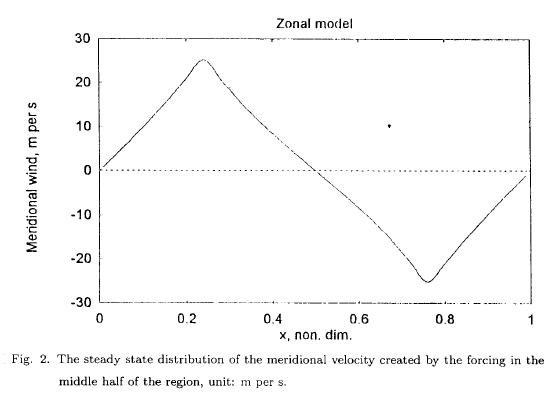
Since fluid is added to the central part constantly and removed in the other part of the region, we would expect that the central part has a fluid level above the average, while the geopotential in the other parts then will be negative, since the net contribution vanishes. Figure 3 shows that also these expectations are correct. The maximum value is more than 8000 m² s^-2 (corresponding to a height difference of about 800 m) with equally large negative values.

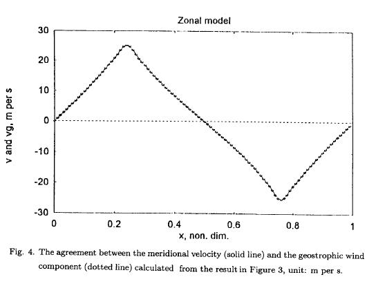
The values after 480 hours of integration represent a steady state. In this state the values of the zonal velocities are quite small indicating that both the nonlinear term and the dissipation term are very small. It is then seen from the first equation of motion that the motion can have a quasi-balance steady state determined by the x-derivative of the geopotential and the Coriolis term, but this is of cource identical to a geostrophic adjustment. The geostrophic meridional wind component was computed from the geopotential in the asymptotic steady state. Figure 4 contains both the real meridional wind component and the geostrophic meridional wind component indicated by points. It is seen that we have obtained a geostrophic adjustment with good accuracy.

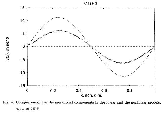
The nonlinear terms in the model equations give a definite contribution to the magnitude of the results in the cases treated above. If one were to disregard all the nonlinear terms in the three basic equations for the model, it is straightforward to calculate the steady state of the linear equations. The linear equations in wave number space are given in equation (3.1).

The steady state solutions are easily obtained by solving the last equation for u(n), whereafter the second equation gives v(n) and the first equation will provide the steady state solution for the geopotential. These solutions are given in equation (3.2). They are valid for all n and may be used to calculate the three variables as functions of x. The steady states for the linearized equations may then be compared with the solutions obtained by numerical integrations of which a couple of examples have been shown at the beginning of this section.

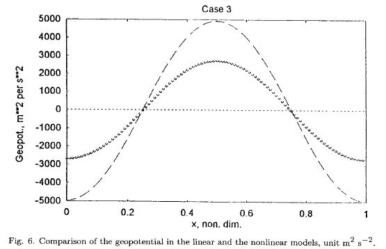
Figure 5 shows the comparison between the meridional wind components in the nonlinear and the linear models, while Figure 6 contains the comparison for the geopotential. A distinct difference between the two sets of solutions is seen in Figure 5 and 6 indicating that the nonlinear equations need to be used to obtain a more realistic geostrophic adjustment.

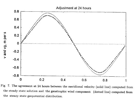
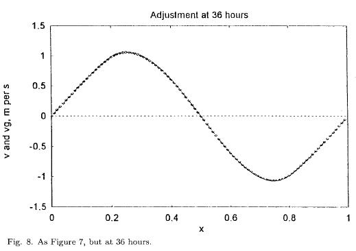
So far we have considered the asymptotic steady states obtained after rather long integrations with respect to time. One may, however, ask if geostrophic adjustment appear before the steady state is reached. To investigate this question a number of shorter integrations with respect to time was carried out and comparisons were made between v and v_g. In the first part of the integration the geostrophic meridional components oscillates around the meridional component computed from the model. An example is shown in Figure 7 where the geostrophic component has a smaller amplitude than the meridional wind component from the model after 24 hours of integration. However, after an integration of 36 hours the two components are almost identical as seen from Figure 8. Thereafter, oscillations of the geostrophic wind around the model meridional wind component continues, but the difference in magnitude is very small. We may therefore say that the essential part of the geostrophic adjustment has taken place within the first couple of days.

While the model described above is based on using sine functions for the velocity components and cosine functions for the geopotential and the forcing, it may be of interest to show that these special results have general validity by introducing full Fourier-series for all variables. When this is done we get twice as many equations with additional sums to evaluate, but the more general equations are of the same type as the equations listed for the more special cases. No new results are found from these integrations.

 

4. The model equations for the meridional case

The early investigations of geostrophic adjustment considered variations in the south-north directions using a beta-plane to model the variation of the Coriolis parameter. We shall treat this case in a way analogous to the treatment in Sections 2 and 3. The nonlinear terms in the equations of motion are now the advections by the meridional velocity components, and the possible geostrophic adjustment appears in the second equation of motion. Similarly, the continuity equation contains the advection by the meridional velocity and a divergence term containing only the y-derivative of the meridional velocity. The basic equations for this case are given in (4.1).

The Coriolis parameter is denoted by f. It is variable in the present case. It is most convenient to model variations in the Coriolis parameter in analogy with the beta-approximation, but paying attention to the fact that the numerical integrations with respect to time are carried out in the spectral domain. It is thus most convenient to write the Coriolis parameter in the form given in (4.2).

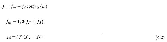
In (4.2) f_N and f_s are the values of the Coriolis parameter at the northern and southern boundaries of the region used for the numerical integrations.

The equations in (4.1) are transformed into the spectral domain. In doing so we use sine series for the two wind components and a cosine series for the geopotential and the forcing function. The three spectral equations may then be written as shown in (4.3).

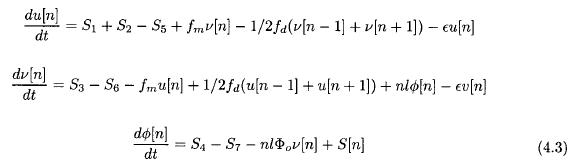
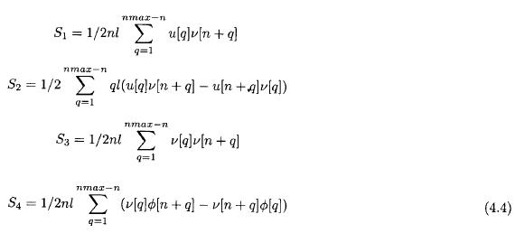
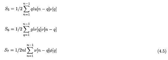
The seven sums entering the equations are defined in (4.4) and (4.5).

The spectral equations are integrated as in the previous case starting from rest and with a specified forcing. It is also in this case necessary to integrate over many hours to come close to a stationary state.

 

5. Results for the meridional case

The first case has a forcing depicted in Figure 9 calculated by summing the 20 Fourier components from the initial assumption that S is positive and constant in the southern half and negative and constant in the northern half. We notice that the limited number of admitted components give a smaller scale wavy pattern.

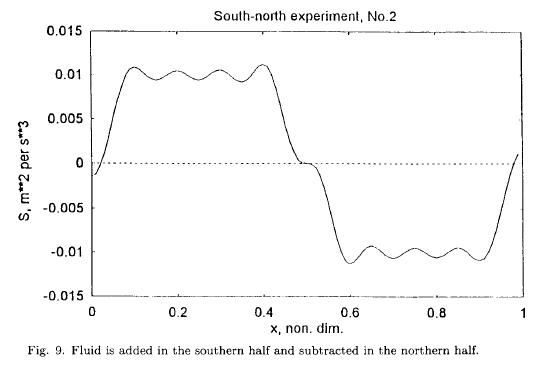
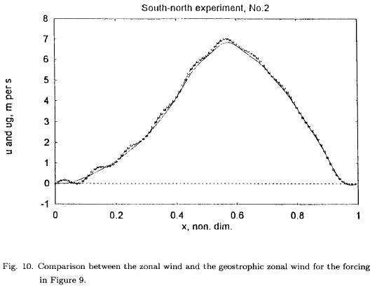
Figure 10 gives the resulting zonal wind components. The dotted curve is the geostrophic u-component computed from the asymptotic value of the geopotential and using f-values as specified in (4.2). Once again we notice that a geostrophic adjustment has taken place during the integration with respect to time.

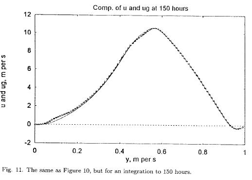
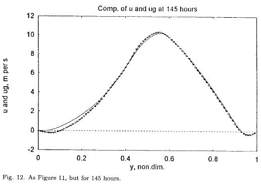
It was also investigated in the meridional case how long a numerical integration needs to be in order to secure a geostrophic adjustment. It turns out that a longer time is needed in the meridional case than in the zonal case. Weak oscillations appear, especially in the region close to the southern boundary and probably due to the small values of the Coriolis parameter in this region. In Figure 11, valid at 150 hours, it is seen that the largest difference is observed close to the southern boundary, where the geostrophic wind (dotted curve) is larger than the u-component in the model. Five hours before at 145 hours, see Figure 12, the situation is the opposite. These minor differences disappear later in the integration, but while the adjustment time in the zonal case was of the order of a couple of days, it is larger in the meridional case.

 

6. A two-level primitive equation model

While the models used above are the most convenient for simple integrations, it may be worthwhile to design an equally simple case using a two-level primitive equation model, where the upper level is at 250 hPa and the lower at 750 hPa. We select the zonal case for this purpose. We shall use the boundary condition at the top of the atmosphere and at the 1000 hPa level that the vertical p-velocity is equal to zero at both levels. Applying the continuity equation at the upper and the lower level in the two-level model and disregarding the y-derivatives we find the equations given in (6.1).

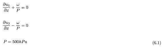
where P=500 hPa.

Setting u₁ = u_* + u_T and u₃ = u_* - u_T we obtain by addition and subtraction the results given in (6.2).

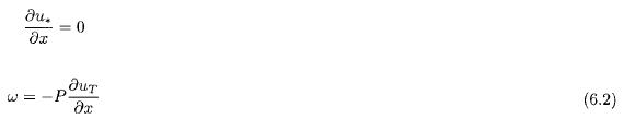
From the first of these equations it is seen that u_* is a constant. Such a value will give a constant transfer in the x-direction. We shall use u_* = 0. The second equation indicates how we can eliminate the vertical p-velocity from the equations. With these remarks we may write the model equations in the form given in (6.3).

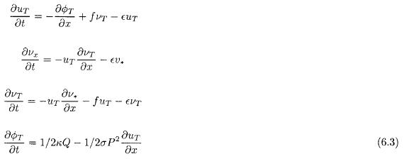
As in the previous case the equations are transformed to wave number space using the same kind of sums as before, i.e. sine functions for the velocity components and cosine functions for the geopotential and for the heating appearing in the thermodynamic equation. Each of the nonlinear terms will create finite sums of the same kind as experienced in the shallow water model. The resulting equations are shown in (6.4).

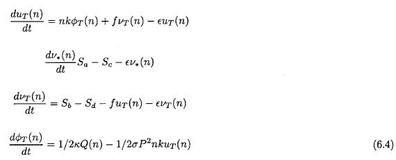
Four sums enter the equations originating from the nonlinear terms in the field equations. They are determined in the same way as before by calculating the triple integrals containing the trigonometric functions. The sums are given in (6.5).

The equations in (6.4) are integrated with respect to time using the same procedure as in the previous cases. We shall finally mention that since u_* = 0 the equation of motion for this variable is reduced to a diagnostic equation from which one may determine the geopotential at the 500 hPa level.

 

7. Results from the two-level model

The model integrations start fron a specification of the components Q(n) determining the x-variation of the heating. All spectral components for the velocities and the thermal geopotential are set to zero at t = 0. The total number of components for each dependent variable are set to n_max = 20.

If we reach a geostrophic adjustment it will, as seen from the first equation of motion, be a balance between the terms containing v_T and the derivative of the thermal geopotential. In addition, it is required that the dependent variables u_T and v_* are small in the steady state or at a time, where the geostrophic adjustment has taken place with reasonable accuracy.

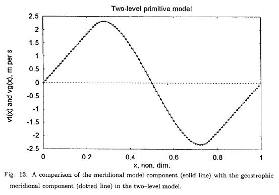
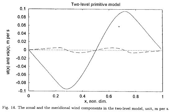
We will limit ourselves to present a single case. The heating is positive in the central region and negative elsewhere. We may think about a winter situation with continents for small and large values of x with an ocean between the continents. The model was integrated for 1000 hours at which time the model is close to a steady state. Figure 13, containing the velocity component v_T and the geostrophic component calculated from the thermal geopotential, indicates a complete balance. Figure 14 contains the curves of u_T and v_s as functions of x. It is seen that both of them are small compared with v_T as seen from a comparison between Figure 13 and Figure 14.

 

8. The problem in two dimensions

The cases treated so far have been essentially one-dimensional, where one of the components of the horizontal wind become quasi-geostrophic, while the other component remains small. These cases were treated using spectral expansions of the variables.

One may then ask if the same kind of model can be used in two dimensions to illustrate a geostrophic adjustment. The case is treated on the beta plane in a rectangular region with length L and width D. The standard equations for the case are given in (8.1), where the forcing as before is introduced through the continuity equation.

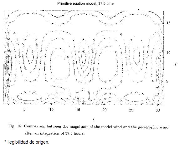
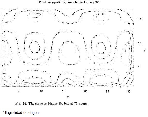
It was decided to integrate these equation from an initial state of no motion and with a flat upper surface. The forcing is given in a Newtonian form and specified in advance and kept constant during the integration with γ = 1.0 x 10^-6 s^-1. For e the value is 4.0 x 10^-6 s^-1. The integration is carried out using centered finite differences in space and time. The boundary conditions are v = 0 at the boundaries to the north and the south. It follows from this boundary condition that u is geostrophic at the same boundaries. Periodic conditions are applied at the western and eastern boundaries. The grid size is 280 km. The time step is 5 minutes, and the dimensions of the total grid is (0,31) in the x-direction and (0,17) in the y-direction.

In the case used for illustration the forcing was specified in the form given in (8.2).

At the end of a time-integration the geostrophic components were calculated in each grid point from the predicted values of the geopotential. The magnitudes of the geostrophic wind vector and the wind vector in the model are compared. Figure 15 shows the comparison at 37.5 hours. It is seen that the geostrophic adjustment process has started, but a close agreement is not observed. Figure 16 is valid at 75 hours. At this time a good agreement is found in the interior of the region. One may also observe that the agreement is better in the northern part of the region, where the Coriolis parameter is large.

 

9. Concluding remarks

The main purpose of the present paper is to show that a geostrophic adjustment takes place using models based on the primitive equations for the horizontal velocity components and the continuity equation for a homogeneous atmosphere with a free surface. A forcing, simulating the heating of the atmosphere, is added to the continuity equations. Two cases are treated. In the first case we use variations in the east-west direction. The meridional wind component (v) adjusts to the changes in the geopotential in such a way that it becomes geostrophic, while the u-component is small.

In the second case we keep the variations in the meridional direction. It is necessary to include the variation of the Coriolis parameter in these examples, where the u-component becomes geostrophic, while the v-component is small when the adjustment has taken place.

It has been shown that the nonlinear terms in the model equation give a contribution to the steady state such that the quasi-geostrophic steady state obtained by the model integrations is different from the one obtained from linear considerations. The magnitude of the forcing determines the strength of the wind components in the quasi-geostropic balance for the same value of the dissipation coefficient.

It should be noted that no attempts have been made to get realistic zonal and meridional distributions of the resulting wind components. The purpose is solely to describe the adjustment process.

The same conclusion is reached, when we apply a simplified version, containing variations in the x-direction only, of a two level primitive equation model based on the two equations of motion, the thermodynamic equation and the continuity equation.

The two-dimensional case of the first model is treated in Section 8.

The present investigations are different from other treatments of geostrophic adjustment, because both forcing and dissipation are included in the models. It would of course also be possible to use a model of the same kind with forcing in both the zonal and the meridional directions. However, the simpler models used here give a better picture of the process, because only one of the two wind components adjust to an almost geostrophic equilibrium, while the other component remains small. The adjustment process is essentially finished after a certain time interval which is relatively short compared to the time it takes to reach the final steady state.

APPENDIX 1

APPENDIX 2

 

REFERENCES

Bolin, B., 1953. The adjustment of a nonbalanced velocity field towards geostrophic equilibrium in a stratified fluid, Tellus, 5, 373-385.         [ Links ]

Blumen, W., 1972. Geostrophic adjustment, Rev. of Geophysics and Space Physics, 10, No.2.         [ Links ]

Cahn, A., 1945. An investigation of the free oscillations in a simple current system, Jour, of Meteor., 2, 113-119.         [ Links ]

Kibel, E. A., 1955. On the geostrophic adaptation of atmospheric motion, Daklad USSR Academy of Sciences, 106, No.1, 60-63 (in Russian).         [ Links ]

Kuo, H. L., 1998. A new perspective of geostrophic adjustment, Dynamics of Atmospheres and Oceans, 27, 413-437.         [ Links ]

Obukhov, A. M., 1949. On the problem of geostrophic wind, Edz. USSR Academy of Science,         [ Links ] Ser. Geogr. and Geophys., 13, 281-306.         [ Links ]

Rossby, C. -G., 1937 and 1938. On the mutual adjustment of pressure and velocity distribution in certain simple current systems, I, II, Jour. of Marine Res., 1, 15-27 and 239-263.         [ Links ]

Wiin-Nielsen, A., 1999. Steady state and transient solutions of the nonlinear forced shallow water equations in one space dimensions, Atmósfera, 12, No.3, 145-159.         [ Links ]

Winninghoff, F., 1968. On the adjustment toward a geostrophic balance in a simple primitive equation model with application to the problem of initialization and objective analysis, Ph.D. Diss, UCLA, 161 pp.         [ Links ]