A note on nonlinear aspects of large-scale atmospheric instabilities

 

A. Wiin-Nielsen

The Collstrup Foundation, The Royal Danish Academy of Sciences and Letters H. C. Andersens Blvd. 37, DK-1553 Copenhagen V, Denmark

 

(Manuscript received June 5, 2000; accepted in final form Oct. 6, 2000)

 

 

RESUMEN

Para ilustrar las inestabilidades y el comportamiento a largo plazo de procesos barotrópicos-baroclínicos, mezclados en modelos sin disipaciones de fricción y forzamiento, se usan: un simple modelo baroclínico con transporte de momentum, un modelo baroclínico sencillo con sólo transportes de calor y un modelo con ambos transportes, de momentum y calor.

Mientras que las inestabilidades de tales modelos son bien conocidas mediante estudios analíticos de las ecuaciones lineales de pertubación, es claro que estos estudios no dan información sobre el comportamiento a largo plazo, que pudieran ser estudiados sólo por ecuaciones no lineales. Las integraciones lineales de las ecuaciones no lineales de orden bajo, serán empleadas para ilustrar el comportamiento a largo plazo, de los dos modelos.

Los aspectos principales de los procesos atmosféricos energéticos observados, pueden reproducirse por modelo general de orden más bajo, usado en este estudio. Este modelo contiene transportes de calor sensible y momentum por eddies que están incluidas en el modelo. Con el fin de reproducir el diagrama atmosférico-energético basado en los estudios observacionales, es necesario incluir disipaciones de fracción y de calor.

Los últimos dos procesos serán excluidos en el estudio presente con el fin de obtener el comportamiento a largo plazo en modelos sin forzamiento. Las integraciones de los diversos modelos indicarán que se observa un comportamiento casi periódico de largo plazo, con escalas de tiempo más bien grandes. Las variaciones casi periódicas se obtienen a partir de estas dos iniciales con valores moderados de los parámetros zonales.

 

ABSTRACT

A barotropic model with momentum transport, a simple baroclinic model with transports of heat only and a baroclinic model with both momentum and heat transports are used to illustrate the instabilities and the nonlinear longer term behavior of barotropic, baroclinic and mixed barotropic-baroclinic processes in models without forcing and frictional dissipations.

While the instabilities of such models are well known through analytical studies of the linear perturbation equations, it is obvious that these studies give no information on the long term behavior which can be studied only by nonlinear equations. Numerical integrations of low order nonlinear equations will be used to illustrate the long term behavior of the two models.

The main aspects of the observed atmospheric energy processes may be reproduced by the most general low-order model used in this study. This model contains meridional transports of sensible heat and momentum by the eddies which are included in the model. To reproduce the atmospheric energy diagram based on observational studies it is necessary to include heating and frictional dissipations. The latter two processes will be excluded in the present study in order to obtain the long term behavior in non-forced models. The integrations of the various models will indicate that a long-term almost periodic behavior is observed with rather large time scales. The almost periodic variations are obtained from initial states with moderate values of the zonal parameters.

 

1. Introduction

The creation of baroclinic and barotropic waves has been demonstrated by using the perturbation methods in which linear equations for infinitesimal disturbances on a zonal state has been solved determining the exponential growth of the perturbations under certain conditions. The classical papers on the subject are by Charney (1947) on baroclinic instability and by Kuo (1949). Numerous studies, too many to reference, have since then been produced using simpler baroclinic models and various steady states. The methodology used in perturbation studies leads to solutions which are valid for a very short time interval due to the fact that the disturbances have been assumed to be small in order to permit the linearization of the equations. On the other hand, the solution obtained in the unstable cases has an exponential growth.

When nonlinear models are used, it is possible to select cases of (linear) instability and perform a time integration of the nonlinear model equations which will show what will happen over a longer time span. The main purpose of the present paper is to show some examples of the behavior of growing waves in barotropic and baroclinic models.

The models that will be used are low order models containing a few spectral components. Such models are very convenient for long term integrations. The fact that the models contain only a few components in the meridional and zonal directions exclude on the other hand such processes as the cascade of energy to smaller and larger scales due to the nonlinear interactions between waves of different wave numbers. The cascade processes are important because they carry energy to the smaller scales where the frictional processes take place. Other types of models are used to simulate the cascade processes (Wiin-Nielsen, 1999).

The two low-order models to be considered in this study have been used for other purposes on earlier occasions. The barotropic low order model is described in details by the author (Wiin-Nielsen, 1961), while the barotropic-baroclinic model was used for several studies (Marcussen and Wiin-Nielsen, 1999). The first of these two models contains momentum transport only, while the other model contains both momentum and heat transports. The baroclinic model is a special case of the two-level, quasi-nondivergent models. Since the models have been presented before, we shall refer the reader to the quoted papers for details of the models.

 

2. The barotropic case

The basic model used in the study is the barotropic vorticity equation modified by the addition of an estimate of the divergence obtained from the continuity equation for a homogeneous fluid with a free surface. The basic equation is given in (2.1).

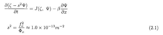
where the parameter s² measures the intensity of the divergence. It has been evaluated as usual at 45 degrees of latitude. The constant value of the geopotential is 10⁵ m² s^-2 corresponding to the approximate height of the troposphere. ζ is the relative vorticity, Ψ the streamfunction and β the meridional derivative of the Coriolis parameter.

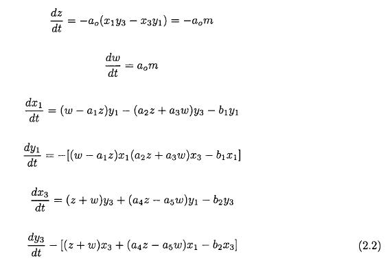
The starting point is the six equations for the low order model described in detail by Wiin-Nielsen (1961) and modified by the divergence term. These equations could be used for long term integrations. However, Thompson (1987) showed for an extremely simple two-level baroclinic model that the basic equations for the model could be replaced by a new, but equivalent set of equations expressed in terms of the zonal parameters, the kinetic energies of the eddy components, the eddy transport of sensible heat by the two eddies incorporated in the model and a final dependent variable expressed as the scalar product of the 500 hPa wind and the thermal wind in the two-level model. With this in mind it was investigated, if a similar result could be obtained for the barotropic case. If possible, the dependent variables might be the two components describing the zonal flow, the kinetic energies of the two eddies, the momentum transport and possibly an extra variable corresponding to the scalar product mentioned above. The basic equations may be written in the form shown in (2.2), where the two zonal components are denoted by z and w, while the parameters describing the eddies are x₁, y₁ and x₃, y₃. These expressions are identical to those appearing in the paper by the author (Wiin-Nielsen, 1961) except for the addition of the divergence term.

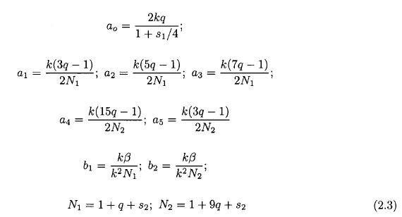
In order to write the coefficients in a brief form it is convenient to introduce some notations. We denote the west-east length of the rectangular region on the beta plane by L and the south-north width by D. With q = λ²/k², s₁ = s²/λ² and s₂ = s²/k², where k = 2π/L and λ = π/D, we may write the coefficients as given in (2.3).

The divergence effect is expressed through the two coefficients s₁ and s_2. If both of the parameters are zero, the model becomes purely barotropic.

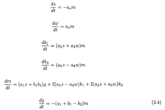
In (2.2) we have introduced the notation M = x₁y₃ — x₃y₁ as the variable measuring the momentum transport. We use then the same technique as Thompson (1987) and arrive finally at the set of equations given in (2.4). As expected we find that a new variable appear. It is denoted by g = x₁y₁ + x₃y₃. The parameter g is proportional to the scalar product of the eddy winds of the two eddy components.

In addition .to these variables we find k₁ and k₃ which are measures of the kinetic energy in the two wave components. The dimension of the zonal components (z and w) is m per s, while the four eddy variables have the dimension m² per s².

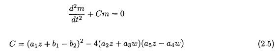
The new model-equations are easier to handle, and they relate physical quantities to each other. Consider the special case where the two zonal components z and w are constants. This will permit us to derive a single second order equation for the momentum transport by differentiating the fifth equation with respect to time and insert from the third, fourth and sixth equations. The result is given in (2.5).

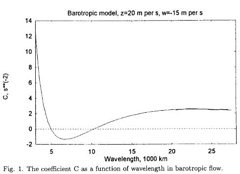
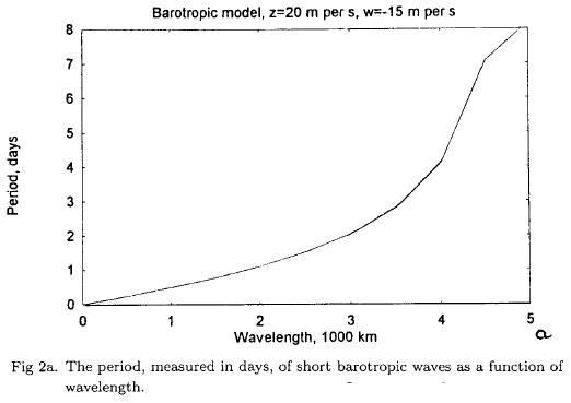
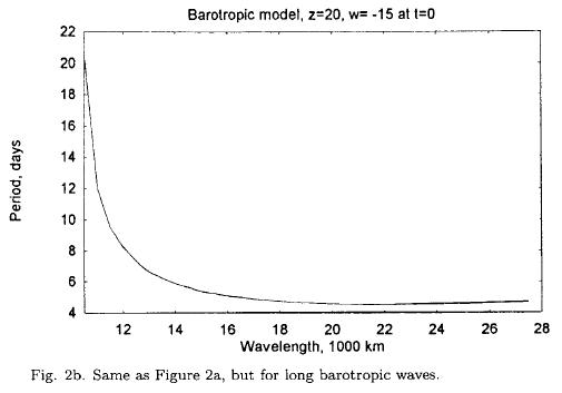
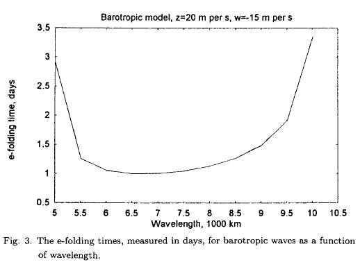
The type of solution of (2.5) depends on the sign of the coefficient C. If C is positive, we have trigonometric solutions, while a negative C indicates exponential solutions. C depends on the constant values of z and w, on the beta effect and on the dimensions of the rectangular region. For a given specification of z and w it is a second degree polynomial in z and w. Figure 1 shows C as a function of wavelength, if z = 20 m per s, w = —15 m per s and D = 7000 km. It is seen that positve values occur for L < 5000 km, while negative values are found for 5000 km < L < 10000 km. For L > 10000 km we find positive values. The result is thus a demonstration of the stability of the low order barotropic model. Figure 2a shows the period as a function of wavelength for the short waves, while Figure 2b gives the periods for the long waves. The period is small for very short waves, but increases to more than a week for a wavelength of about 5000 km. For the long waves the period decreases with the wavelength, and the period for very long waves is 4-5 days. Figure 3 displays the e-folding times for the unstable waves. The e-folding time becomes as small as 1 day for the most unstable waves. The results are obtained for constant values of the two variables describing the zonal flow. In the following we shall investigate the behavior of the model using long term integrations of the nonlinear equations.

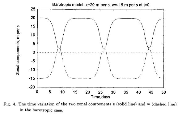
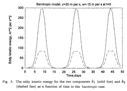
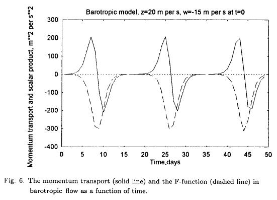
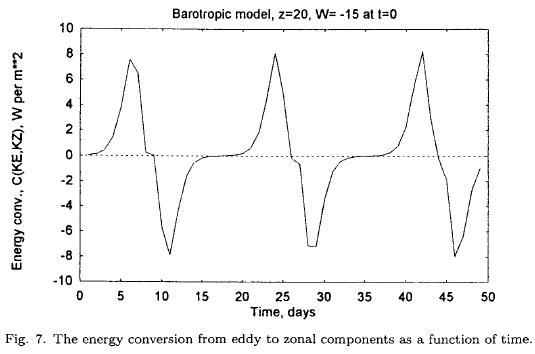
The nonlinear equations, containing no forcing and dissipation, will permit interactions between the zonal flow and the eddies. From an energetical point of view we have only the energy conversion between the zonal flow and the eddies, i.e. C(K_E, K_Z). The integrations have to be carried out with good accuracy to satisfy the conservation properties of the equations such as the conservation of the sum of the two zonal components (z + w = constant). The integration have in some cases been made with Heun's scheme. In other cases of high instability it was either necessary to use a small time step in Heun's scheme or a high accuracy formulation of the Runge-Kutta scheme. The examples have the same basic parameters as the stability investigations described above. In the following example we have selected L = 7000 km and D = 7000 km which is close to the most unstable wave. At t = 0 we have used z = 20 m per s and w = —15 m per s, while the remaining variables were set to a small value of 0.1 m² per s². Since we expect a long period, the integration was carried out for 50 days. Figure 4 contains the zonal components, z and w as a function of time. After a while z decreases and w increases. The sum of the two variables should be constant. With the values used in the example the sum should remain at 5.0 m per s. The sum was evaluated at each time step to measure the accuracy of the numerical integration, and it was found that the conservation was maintained during the whole integration. The variation is obviously periodic. As it can be seen the period is close to 18 days. As shown by the author (Wiin-Nielsen, 1961) the zonal kinetic energy has a minimum when z = w, or, in other words, the available zonal kinetic energy is proportional to (z — w)². Figure 4 shows that this happens when z = w = 2.5m per s. Figure 5 shows the eddy kinetic energies of the two waves displaying the same periodicity. The energy k₁ is considerable larger than k₃. Figure 6 contains the momentum transport (m) and the scalar product (g). They are interrelated by the last equation of the system. It is seen that g decreases as long as m is positive. For negative values of m the parameter g will increase. Figure 7 shows the energy conversion C(K_E, K_Z) as a function of time. It oscillates between positive and negative values and reaches values as large as 8 W per m².

Several integrations of the barotropic system, using other initial states, have been carried out. Integrations for very short and very long waves indicate that the periodic variations are present also in these cases, but the amounts of energy in the two eddy components are much smaller than for wavelengths of the order of 7000 km using the same initial states as given above. The results of the stability analysis were also tested by making several integrations with wavelengths a little smaller and little larger than 5000 km.

 

3. A simple baroclinic model

Turning the attention to baroclinic models it may be an advantage to start with a relatively simple case. Such a simple model was considered by the author (Wiin-Nielsen, 1992). The meridional variation of the thermal zonal flow is given by a single trigonometric function, and the same is true for the eddies. The streamfunction is given in (3.1).

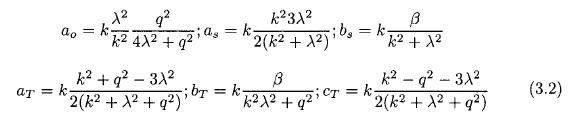
The definition above is used for the streamfunction at 500 hPa (subscript 's') and for the thermal streamfunction (subscript 'T'), where the thermal streamfunction is half the difference between the streamfunctions at 250 and 750 hPa. The coefficients are listed in (3.2). We should recall that k = 2π/L and λ = π/D, where L is the length and D the width of the channel.

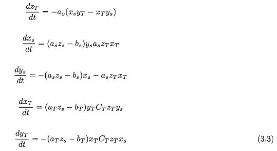
The model equations are given in (3.3), where it should be noted that the mean zonal wind at 500 hPa does not change with time reducing the model to have five dependent variables.

The five equations may be integrated with respect to time as was done by the author (Wiin-Nielsen, 1992) in the case with heating and dissipation. It is, however, also possible in this case to replace the five equations listed in (3.3) by a new set using a procedure similar to the one used in the barotropic case. We note first of all that the quantity in the parenthesis in the top equation is the amplitude of the transport of sensible heat. The quantities, listed in (3.4), are introduced in analogy with Thompson (1987). The present model is not identical with Thompson's model, but the same technique can be applied.

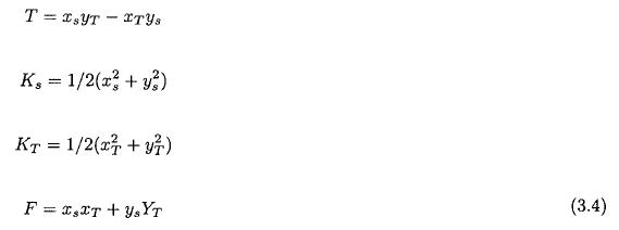
The physical meaning of these quantities are, in addition to the heat transport, that K_s and K_T are measures of the kinetic energy of the eddies at 500 hPa and in the thermal flow, while F is proportional to the scalar product of the horizontal winds at 500 hPa and in the thermal field. A quantity similar to F is found in the model by Thompson (loc. cit). It may be called the interaction term since it, just as the transport of sensible heat, involves both the mean flow and the thermal flow.

After some algebra we arrive at the new set of equations given in (3.5).

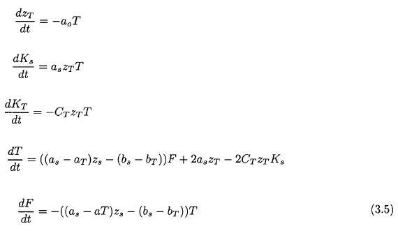
These equations contain the same information as the original model equations, but they are easier to handle from an algebraic point of view and also more convenient for numerical integrations with respect to time. With the assumption that z_s and z_T are given constants we may make a perturbation analysis. When the heat transport equation is differentiated with respect to time followed by insertion from the other equations we arrive at a single, second order equation in T. It is given in (3.6).

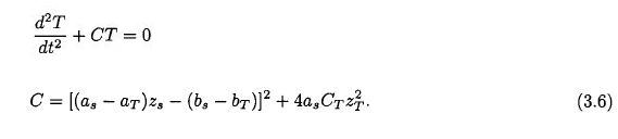
The equation in (3.6) is convenient for a stability analysis in which z_s and z_T are constants determining the zonal flow in the model. Under this assumption C depends on the length and the width of the adopted region and on the beta effect. If C > 0 the solutions to (3.6) are trigonometric functions indicating stability. In the other case (C < 0), the solutions are exponential functions in time giving instability. It is obvious that a necessary condition for a negative value of C is that a_s and c_T are of opposite sign. However, the possible region of instability is most easily obtained by calculating C as a function of the zonal wavelength for fixed values of the width of the channel, z_s and z_T.

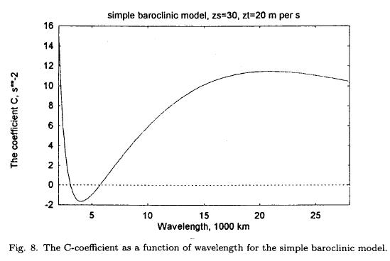
Figure 8 gives an example of a calculation of C = C(L) computed with D = 10000 km, β = 1.6 x 10^–12 m^-1 s^-1 and a value of q² = 4.0 x 10^-12 m^-2. It is seen that C(L) is negative in a relatively small region around a wavelength of 4000 km, while C(L) > 0 for all other wavelengths.

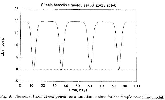
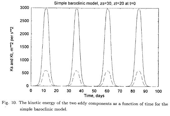
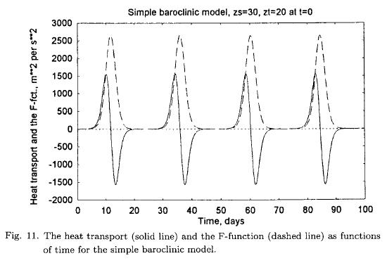
The next step is to make a numerical integration of the equations given in (3.5). A basic wavelength of 3600 km is chosen. The initial state is set to reasonable values of z_s and s_T , while small values are used for the four dependent variables related to the eddies of the model. It turns out that an integration of 100 days is necessary to determine the period of the changes in the variables. Figure 9 shows the variation of s_T with respect to time. The instability is seen after an integration covering about one week. The zonal flow decreases indicating a conversion from the zonal flow to the eddies. As can be seen from Figure 10 the kinetic energies increase for each of the eddy components with the larger values in the 500 hPa flow. The intensity of the eddies reaches a maximum whereafter they decrease to infinitesimal values. The same variations take place repeatedly as the integration is extended in time. Figure 11 contains the heat transport and the F-function as functions of time. These two functions are closely interrelated as one can see from the fifth equation for the model. As long as the heat transport is positive, F will increase. A decrease of the F-function starts when the heat transport turns negative. Note that the coefficient in the fifth equation is negative in the present case.

The case illustrated in Figures 9, 10 and 11 is chosen close to the maximum instability as can be seen from Figure 8. If L is selected outside the interval of instability very small changes are found in the eddy quantities.

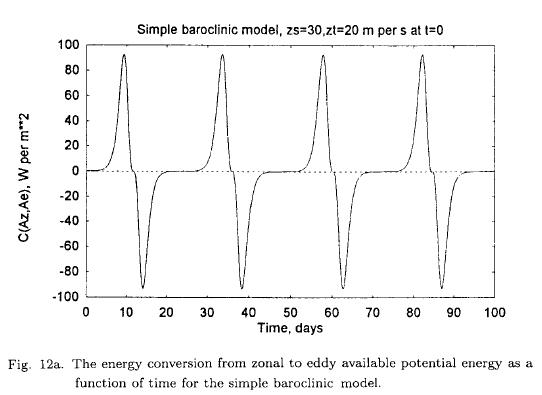
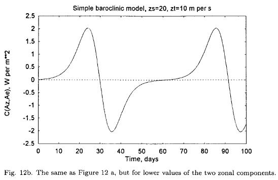
Figure 12a shows the energy conversion C(Az, Ae) as a function of time. When the wave is growing the energy conversion is positive, but it changes sign during the time where the wave amplitude is decreasing. As can be seen from Figure 12a the chosen example is very extreme. This is due to the selection of extreme values of z_s and z_T . More moderate values such as z_s = 20 m per s and z_T = 10 m per s will give more realistic values of the energy conversion as can be seen from Figure 12b indicating also a much longer period.

The period for the example treated above is close to 24 days as can be seen on all the figures. Periods of the same order of magnitude is found in other examples, but the result is very dependent on the choice of the wavelength in the region of instability and on the initial values of the two parameters determining the zonal flow.

 

4. The barotropic-baroclinic case

The model applied in this section has been described in detail in the paper by Marcussen and Wiin-Nielsen (1999), where several cases including heating and dissipation were presented. It is a two-level, quasi-nondivergent model with six components at each level resulting in twelve equations to be integrated. It is realistic from the point of view that it contains both transports of sensible heat and momentum, and it can be seen as a generalization of both the barotropic model treated in Section 2 and the simple baroclinic model used in Section 3.

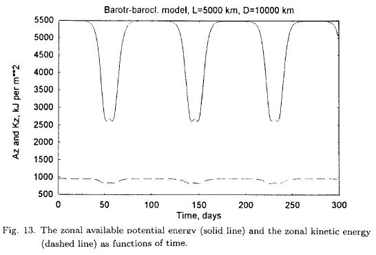
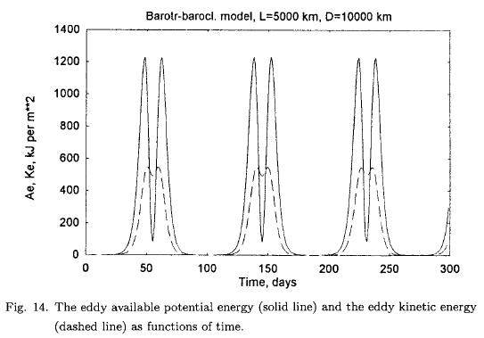
In the following example, the numerical integrations are carried out using the basic equations (Marcussen and Wiin-Nielsen, 1999) disregarding all terms related to heating and friction. The zonal wavelength is chosen to be 5000 km, the width of the channel of 10000 km and q² = 4.0 x 10^–12 m^–2. Figure 13 shows the zonal available potential energy (A_z) and the zonal kinetic energy (K_z) as a function of time over a total integration time of 300 days. As with the simpler model we notice periodic temporary reductions of A_z and Kz followed by increases taking the parameter back to its initial value. The changes of these two energy quantities are in phase although the variations of the zonal kinetic energy is much smaller than those for the zonal available potential energy. This behavior indicates clearly that we have an instability of a mixed barotropic-baroclinic nature. The period is about 80 days. Figure 14 contains the eddy available potential energy (A_e) and the eddy kinetic energy (K_e) as a function of time. It is seen that A_e and K_e have a double maximum before both of the variables return to very small values.

 

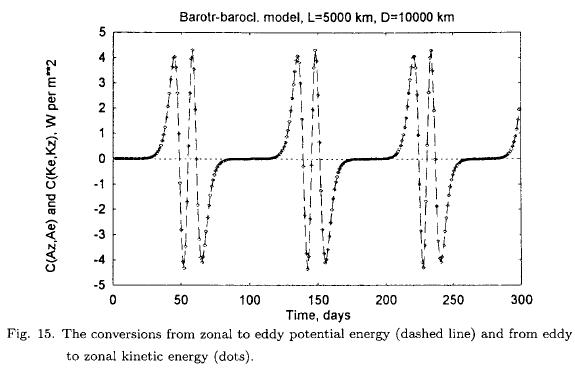
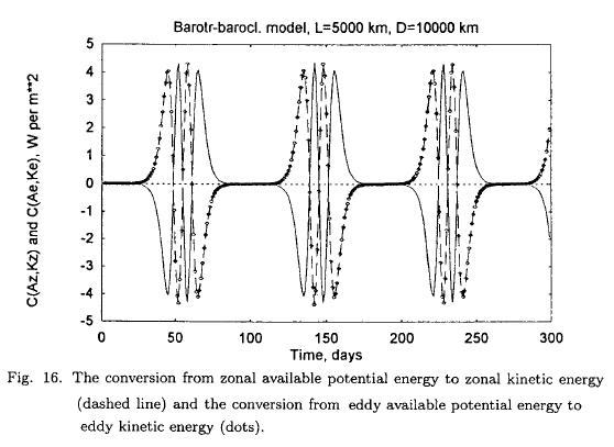
To describe this behavior it is useful to calculate some energy conversions. Contrary to the former models treated in sections 2 and 3 of this paper the present model permits the calculation of all the internal energy conversions. Figure 15 displays the energy conversions C(A_z,A_e) and C(K_e,K_z) computed independent of each other. As can be seen the two energy conversions are identical functions of time. Both of them oscillate between positive and negative values. The largest values are 4 to 5 W per m². Figure 16 contains the remaining two internal energy conversions, i.e. C(A_Z, K_z) and C(A_e, K_e). We observe that these energy conversions have opposite signs, but the same absolute value. Based on these calculations it may be concluded that the energy conversions during half the integration time follow the directions: A_z → A_e → K_e → K_z → A_z, while the conversions follow the opposite directions for the remaining period. The reason for these cyclic changes is of course that these integrations are carried out without any heating and friction. On the other hand, when these processes are included in the model used in this section, it was shown by Marcussen and Wiin-Nielsen (1999) that the directions of generations, conversions and dissipations are in agreement with the directions as found from observational studies.

 

5. Concluding remarks

The main purpose of the note is to investigate the stability of a few simple models. For the barotropic and the simple baroclinic model it has been demonstrated that the equations for the basic low order model may be transformed to a different set of equations from which the stability criteria can be easily computed. The long term behavior of the models have been demonstrated using long integrations of the model equations. A result of these integrations is the determination of the length of the period dominating the behavior of the long term integrations of the model equations. The energetical behavior of the models has also been determined.

The most general model contains the transports of sensible heat and momentum. The model equations have been integrated with respect to time. In addition to the determination of the period for the long term behavior it has been possible to illustrate the energetical behavior of the model. It is found that energy conversions go through a cyclic change where a given conversion changes direction during half of the period for the long term behavior. The reason for this behavior is that the model contains neither heating nor friction. It is thus the inclusion of these two processes that determines an energy diagram in agreement with observational studies.

 

REFERENCES

Charney, J. G., 1947. The dynamics of long waves in a baroclinic westerly current, Jour. of Meteorology, 4, 135-162.         [ Links ]

Kuo, H. L., 1949. Dynamic instability of two-dimensional, non-divergent flow in a barotropic atmosphere, Jour. of Meteorology, 6, 105-122.         [ Links ]

Marcussen, P. and A. Wiin-Nielsen, 1999. A numerical investigation of a simple spectral atmospheric model, Atmósfera, 12, 28-43.         [ Links ]

Thompson, P. D., 1987. Large-scale dynamical response to differential heating: Statistical equilibrium states and amplitude vacillations, Jour. of Atmospheric Sciences, 44, 1237-1248.         [ Links ]

Wiin-Nielsen, A., 1961. On short-and long-term variations in quasi-barotropic flow, Monthly Weather Review, 89, 461-476.         [ Links ]

Wiin-Nielsen, A., 1992. Comparisons of low-order atmospheric dynamic systems, Atmósfera, 5, 135-155.         [ Links ]

Wiin-Nielsen, A., 1999. Steady state and transient solutions of the nonlinear forced shallow water equations in one space dimension, Atmósfera, 12, 145-160.         [ Links ]