


 nueva página del texto (beta)
 Inglés (pdf)
 Artículo en XML
 Referencias del artículo
 Enviar artículo por email
 Citado por SciELO
  Similares en
SciELO
Similares en
SciELO 
 Permalink
1. Introduction
Industrial development goes hand in hand with policies dictated by governance. Results of a study by Borratero (2019) in Argentina suggest that the articulation between quality state interventions and local business action oriented to sectoral growth with high degrees of rooting and reciprocity, favored the growing dynamism of the sector analyzed during the 2000s.
Therefore, it is clear that strategic project management is key in industrial development to create environments where appropriate scenarios and guidelines can be generated, enabling objectives and goals to encourage production and productivity growth. Strategic decision-making is seen as a complex system of interrelationships that affects other production processes and indicators.
This particular case study must determine which investment projects will be executed in a portfolio.
Thus, implementing portfolio management models is a fundamental tool for strategic decision-making, e.g., standards presented by organizations acknowledged at global level: The Standard for Portfolio Management - Fourth Edition PMI (Project Management Institute), MoP Portfolio Management (Axelos) and the IPMA Competence Baseline (International Project Management Association.)
In these traditional methodologies, interactions between strategic subsystems, projects and production are shown linearly, thus limiting strategic action and decision-making. Traditionally, the process- or product-based analysis techniques that are selected fail to recognize interactions of each of the organizational system’s variables, considered complex environments.
In this sense, the model proposed herein is a new model based on system dynamics (SD). Unlike linear models in which problems are solved maximizing or minimizing the objective function (subject to certain constraints,) the new model proposed is based on equations where the modeled phenomenon is "described using a set of equations that interconnect the behavior of individuals or groups of individuals to the environment they inhabit" (Sterman, 2000, p.45).
The structure of the document consists of six sections. The first one is the introduction to this work. The second section describes the methodology and illustrates the route followed to build the causal model and the flow model. The third describes the results of the models and trials in the Colombian poultry sector. Subsequently, results are discussed; and finally the conclusions of the research are presented.
2. Literature review
This section details the background and presents similar research studies.
In relation to the above, Cardona and Olivar (2017) in their research Modeling and Simulation of Project Management through the PMBOK® Standard Using Complex Networks, conclude that complexity (part of the thinking that dominates project management applied today) is still based on control theories developed -in some cases- in the 1950s. However, problems occur when they are applied unilaterally to all kinds of drafts.
Cardona and Olivar (2017) add that some authors have concluded that the classical perspective has been insufficient to understand the dynamics of complexity. In addition, the authors also state that projects addressing complex situations can be described as complex adaptive systems, with multiple interdependent dynamic components, multiple feedback processes, non-linear relationships and handling hard data (process dynamics) and soft data (dynamic) by the executing team.
In terms of portfolio management, Shojaei and Flood (2017) conducted a study in the Florida Department of Transportation Projects with the aim of developing and validating a stochastic model capable of generating representative flows of future projects’ uncertainty, in order to demonstrate its importance in project portfolio and strategic planning. As a conclusion, the authors affirm that companies must have the ability to focus not only on known projects, but must also bet on uncertain and unknown projects, and that this commitment is key to effective strategic planning in the mid- and long-term of the company's project portfolio.
Similarly, it was found that Perez et al. (2018) in their article Selection and Planning of Project Portfolios with Diffuse Restrictions, incorporated the existence of uncertainty in different aspects pertaining to the project’s decision-making. The researchers proposed a mathematical model based on fuzzy parameters that allows representing information that decision-makers are unaware of, since uncertainty and ignorance in the political, economic, social and legal fields becomes important due to the strong interdependence existing between the projects and the conditions of the environment in which they are developed. Although there are multiple mathematical models, these cannot handle the complexity of real-world challenges if they do not consider uncertainty in their models for dynamic and real-time analysis.
To complement and referring to system dynamics and strategic planning by scenarios, Li et al. (2017) express in their article Research on Investment Risk Management of Chinese Prefabricated Construction Projects Based on a System Dynamics Model, that projects move in environments that are constantly changing and in which different variables intervene. The latest research is steered by the use of system dynamics, used to investigate systems’ social and economic complexities and is based on feedback theory that uses computer simulation technology. In their research, the authors used the system dynamics method to create a risk identification feedback model diagram, and to create a flow chart of the risks associated with precast construction projects in China.
On the other hand, Allington et al. (2018) conducted a study of Complex Socio-Ecological Systems in Mongolia using feedback for the system’s quantitative modeling and planning by scenarios as tools for the interpretation of results compared with the system’s behavior. The result was a conceptual model based on three subsectors that interact with each other: humans, environment and land use. Using that conceptual model, they developed a dynamic model based on differential equations to simulate the scenarios and to be able to compare the projections of the system’s key variables. The authors conclude that the scenario-based simulation helps reveal the behavior of the system’s key variables over time and the interactions between them; and that the use of scenario-planning facilitates interdisciplinary dialogue to obtain and exchange different perspectives on a problem and the way of thinking about it. Moreover, that the use of qualitative scenarios with quantitative simulations helps prevent the system’s behavior against unexpected situations.
In 2018, in Brazil, systems dynamics were used to support complex decision-making process in housing planning for low-income citizens in the city of Florianopolis. The research includes modeling, simulation and participation of stakeholders. The variables used and the interrelation between them were taken per the experience and knowledge of those involved. The model allowed decision-makers to control the most influential variables and different scenarios under future conditions and desired times (de-Oliveira-Musse et al., 2018).
Also Rad and Rowzan (2018) published their article Design of a Dynamic Hybrid System Model to Analyze the Impact of Strategic Alignment on the Selection of the Portfolio of Projects, which presents a model that integrated system dynamics with decision-making to address project portfolio selection. The project portfolio was modeled using four aspects including technology, complexity, innovation and time sensitivity, and the objective was to plan and monitor its progress while assessing strategic adaptation subject to changes in human resources. The result of the sensitivity analysis indicates that the proposed model provides information on strategic alignment’s impact on project portfolio selection. Results of the simulation through system dynamics concluded that the research proposed by the authors supports adequate project selection, contributing in turn with the achievement of the organization’s strategic objectives.
On the other hand, Sarnoe et al. (2018) in the article Use of SSM in Project Management: Alignment of Objectives and Results in Organizational Change Projects, propose the use of the Soft Systems Methodology (SSM) in project management by exploring what happens in real-world organizational change projects when stakeholders appear to agree on a set of initial project goals and end results.
In summary, SSM analyses are used to explore initial objectives and final results’ misalignments throughout the project’s life cycle. Initial results suggest that SSM helps "shade" these misalignments by structuring an unclear complex situation, such as organizational change projects, and that the application of SSM facilitates negotiations, generates debate, understanding and learning. This leads to meaningful collaboration between stakeholders and enables key changes to reflect on potential misalignments. Results also support SSM's analyses of changes in role, standards or value that negatively influence the project's outcome.
Shahabi et al. (2020) in their article Combining Soft Systems Methodology with Interpretive Structural Modeling and System Dynamics for Network Orchestration: Case Study of the Formal Science and Technology Collaborative Networks in Iran, present a study that incorporates the use of SSM and system dynamics to design a model of formal determination of the system of collaborative networks of science and technology in Iran. The authors used SSM to conduct a systematic study of existing stakeholders in a problem with complex structure, based on stakeholders’ perceptions and root definition to illustrate the system, its main variables and the dynamics between them. To facilitate the analysis of the variables, they used system dynamics to produce the design of the final solution-focused model that corresponds to a dynamic model.
The purpose of the research by Kitsios and Kamariotou (2019) Business Strategy Modeling Based on Enterprise Architecture: A State of the Art Review, is to evaluate contemporary issues in existing Enterprise Architecture (EA) modeling frameworks in terms of optimizing business strategy concepts and identifying areas of improvement. Studies were identified using the three-stage literature review methodology suggested by Webster and Watson (2002).
Results showed that a holistic approach is needed due to issues related to the lack of guidelines for modeling business strategy. The article contributes to the existing literature by evaluating current EA modeling languages and their ability to model strategy. In the first place, it is a contribution to the determination of modeling difficulties, as well as to the examination of the ease of use of the language in the context of the strategy. Second, the research provides an overview for professionals looking to develop effective EA modeling projects, as well as for architects trying to solve problems of business complexity.
Danylyshyn et al. (2019) in the article Real Options Method in Investment Project Management published in the International Journal of Innovative Technology and Exploring Engineering, present an investigation in which they argue that a key factor for project management’s success is the existence of a clear predefined plan to minimize risk and deviations, and to strengthen efficient change management (as opposed to process, functional and service level management.).
In addition, Zapata-Ruiz and Oviedo-Lopera (2019) in their Model Study of Simulation of Productivity Alternatives to Support Decision-Making Processes in Companies of the Antioquia Floriculture Sector, analyze the results obtained by intervening a group of five companies in the floriculture sector in Antioquia, Colombia, dedicated to the production of export flowers. The Business Process Modeling (MPN) is applied, enabling the identification and collection of data associated with the critical variables of the production process in its different phases. Subsequently, a simulation of the process is conducted to find out the use of available resources that optimize productivity. Characteristics associated with competitiveness of this type of companies were determined and three scenarios were proposed in which profitability is observed by varying the type of flower harvested, demand and currency exchange (p. 57.).
Similarly, Angarita-Zapata et al. (2019) in their research Expanding Processes and Learning Spaces in Agribusiness with Systems Dynamics (2019), propose a strategy to integrate modeling and simulation with system dynamics in agribusiness training offered by the Institute for Regional Projection and Distance Education at Universidad Industrial de Santander. The design and implementation of the strategy were undertaken through experiment-experiences with teachers and students in the Animal Nutrition Management subject of the agro-industrial program. Said experiences revolved around the use of learning environments in class to complement theoretical knowledge through simulated experimentation that would be closer to real experiences in the field. Experiences-experiments conducted and the proposed strategy make it possible to conclude that learning environments allow the development of decision-making capacities supported by simulation scenarios very close to field reality (p. 169.).
This search evinced scant evidence of the existence of research involving the use of system dynamics in project portfolio management in agro-industrial sectors. Therefore, the objective of this research is a contribution of knowledge with the development of a quantitative portfolio management model based on system dynamics to decrease uncertainty in decision-making processes in terms of efficient allocation of resources to projects in agro-industrial sector’s portfolios.
3. Materials and methods
Research design was structured according to Figure 1.
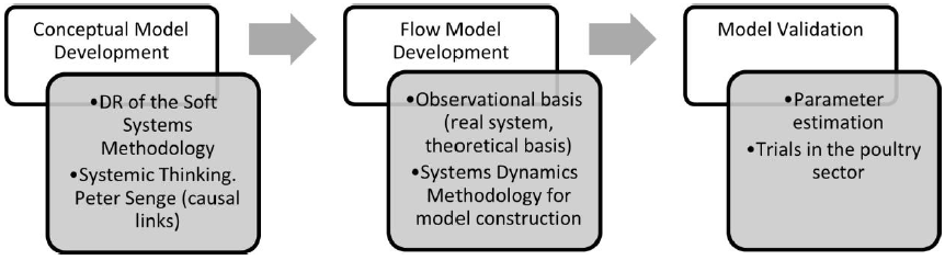
The iterative process of SD modeling comprises different stages for this research, as described below.
The first stage is the system’s description or conceptualization. This stage consists of establishing the model’s purpose and limits, the mode of reference and the nature of its basic mechanisms. In this phase, the system is described and some hypotheses arise as to how the structure generates the problem behavior and difficulties understanding or exchanging information about this behavior, for which it is beneficial to use causal diagrams.
The second stage is the formulation of the model. This entails a rigorous description of the system consisting of translating causal diagrams into equations of levels and rates, as well as into parameter values. Its formulation could reveal inconsistencies that would require modifying the previous description.
The third stage is simulation, which allows testing dynamic hypotheses, knowing the model’s behavior and its sensitivity to external disturbances. “The existence of discrepancies with respect to the real system would require a refinement in the equations” (Serra, 2016, p.122) to verify structural consistency.
The fourth stage corresponds to model testing: Testing the model’s responses to different policies to determine those that drive improvement. Alternatives may come from intuition generated in previous stages, analyst's experience, or from testing automatic and comprehensive parameters. The latter should be the last resource because the modeling process is expected to foster participants’ creativity (Serra, 2016, p. 122).
The following is a description of the different phase of the system dynamics modeling methodology followed by this research.
3.1. Phase of problem identification and behavior analysis
According to Sterman (2000), the key to understanding complex systems is generalization. Therefore, this process must begin by defining the system’s limits per the specific question or questions for which an answer is sought (p. 32.) Consequently, in this first phase the problem must be clearly specified. It begins by collecting information and listing all the variables considered suitable for the system. Subsequently, the associated key variables are identified to the magnitudes whose variation over time we want to study (and that helps define the aforementioned system’s limits,) as well as the feedback of the structure that governs its dynamics. It is convenient to describe them based on the arguments presented by Sterman (2000) for the system’s characteristic behaviors, which he called modes of reference, showing the temporal evolution of the variables.
Sterman (2000) indicates that the reference modes are graphical representations of the behavior patterns of key variables over time. They don't have to necessarily reproduce the observed behavior but they illustrate a behavioral characteristic that is considered interesting. They can refer to both the past and the future, being able to express what is estimated, feared or expected (p. 32.)
Normally the variable is represented on the ordinate axis and time is shown on the abscissa. In some cases, it may be important to show the relationship between the model’s variables. These are useful for checking the bottom structure of the model, for the identification of feedback loops and as a complement to verbal descriptions of behavior.
In the case of System Dynamics, Sterman (2000) points out that quantitative data is not required to capture the dynamics of the modes of reference. When numerical data are not available, the behavior of the variables is made based on the description made and on other qualitative information. It is advisable not to omit important variables for the simple fact that they have not yet been measured or because the data are not easily obtainable (p. 32.) Morlán (2010) suggests the contribution of experts in the area of application, as well as the information of other similar models for the first phase.
This particular research followed the first three steps of the Soft System Methodology to create the conceptual model of feedback loops.
3.2. Soft system methodology (SSM) formulae (Science style)
The guidelines of the SSM are applied to identify the problem situation being studied and the subsequent development of the conceptual model. According to Checkland (1981), this method has a systemic principle because a study is made considering the entire container system located on a level higher in the hierarchy.
Checkland and Poulter (2006) describe the SSM as a methodology for complex problems that resist sharp definitions or structured approaches. It is used to formulate conceptual models for structural thinking in situations where a complex human component is present.
The SSM uses a collection of models and looks like an organized learning system. For his part, Checkland (1981) classifies the individual's perception of a system either as hard (a structured systemic approach) or soft (structured in areas of real world problems that represent multiple visions.) On the other hand, Patel (1995) argues that hard systems can be predicted to some extent while soft systems are unpredictable, confusing, and involve human activity. The SSM explores the idea that people act on purpose, intentional action implies that "something must be done about it." The ultimate end of this process is to improve the problem area. Checkland and Poulter (2006) oppose using the words "problem" and "solutions", they claim that "problem" suggests there is a clearly defined problem, and that "solution" implies that the SSM will fix it. Moreover, they argue that SSM’s objective is to seek different visions in the place of consensus; visions must be desirable and culturally feasible for all stakeholders.
3.3. Real world perceived problem situation
The first activity involves exploring the initial problem situation. Checkland and Poulter (2006) suggest analyzing the problem situation in an unstructured format. The researcher may also experience a problematic situation, leading to assumptions about the nature of the situation. The first step is to formulate the problem situation in terms of entry, transformation and exit.
The second step is to express the problem in terms of a detailed figure in which the problem occurs. The main goal of this is to capture the rationale, culture and relationships. Checkland and Poulter (2006) offer structures, processes and climate, people, problems expressed by people and conflicts. This is a holistic impression of a problem area of interest that is formulated using interviews and existing documents.
• Creation of the model
According to the proposals by the aforementioned authors, the second activity is to perform relevant activities based on the perception of the real world. Each perspective is a guide for the particular model. A model can never be a definitive description of the real world, but rather a representation of the particular perspective desired from the real world. Models are ideal situations. They model a way to visually examine the involutional authenticity of the world.
The PQR formula means: [P (What?) times Q (How?) helps achieve R (Why?)]
A sentence in the form "P times Q helps achieve R" should first be constructed by a SSM practitioner. The PQR formula is used as the development process for the root definition (RD). RD enrichment is achieved by answering questions like: What? How? and Why? Checkland and Poulter (2006) give the transformation formula. The meaning of PQR is P (What?) times Q (How?) helps achieve R (Why?). The key element of this formula is Q, which represents the transformation process. The other two (P and R) are the supporting elements that define Q in the equation. Transformation is the process of converting or achieving the result given a specific input.
• Perceived problem situation of the real world
The second step is the application of the CATWOE model, one of the most popular and fundamental SSM tools for the process of deriving a root definition.
CATWOE means:
C = Customer
A = Actors
T = Transformation Process
W = Weltanschauung (World View)
O = Owner
E = Environmental Limitations
According to Checkland and Poulter (2006), CATWOE analysis is used to articulate the scope and components in a problem situation.
• Root definition (RD)
Following the expository line of the cited authors, RD is a detailed description of the activity formulated to improve analysis efficiency. It is a narrative that describes the problem in terms of the components of PQR, CATWOE, and the evaluation criteria.
3.4. Phase of problem identification and behavior analysis
In this second phase a dynamic or causal hypothesis is elaborated, it implies defining the influences between the system’s elements. When it starts linking causal relationships, a vision of the model is obtained. It is necessary to know what the other variables you want to influence depend on. That is, how the components and the causal relationships between the variables of a system work must be understood.
The result of this phase is the Influence Diagram or Causal Diagram (Causal Loop Diagram -CLD) which shows the basic relationships in the form of loops of feedback along with potential delays. It is important to know that a causal diagram leaves out other characteristics such as information on the simulation time or on the nature and magnitude of the variables. These are obtained in the next phase of mathematical modeling.
3.5. Causal diagram
It is an instrument to show a system’s structure and causal relationships in order to understand its feedback mechanisms on a temporary scale. Basic elements are the variables or factors and the links or arrows. The TO variable is a condition, a situation, an action or a decision that can influence or be influenced by other variables (Morlán, 2010).
One of the fundamental traits of causal diagrams is that they can incorporate qualitative variables, also known as soft variables, which are variables that lack numerical data and include factors such as qualitative characteristics, perceptions and expectations concerning a person or thing. The second element of the causal diagrams can be seen in Figure 2. They are the arrows or links that show a relationship of causality or influence between two variables, so that a change in the origin of the arrow produces a variation in the response the variable.

Two types of influences concur in causal diagrams: positive and negative. The representation of the relationship is expressed by associating a sign with the arrow. Figure 3 shows a positive influence relationship, which means that both variables change in the same sense: If variable A increases or decreases, variable B also increases or decreases.

Figure 4 shows a negative influence relationship with the negative sign, which indicates that the variables at the two ends of the arrow change in opposite direction: If variable A increases or decreases, then variable B decreases or increases (Morlán, 2010).

Figure 4 Relationship of the negative influence. Taken from La Quinta Disciplina por Senge (1995, p. 93).
3.6. Feedback loops or causal circles
The structure of feedback is considered in the study of a system’s behavior. According to Senge (1995) the feedback loops or causal circles represent the dynamic process that moves through a chain of causes and effects to a set of variables that ends up returning to the original cause. Fittingly, a feedback loop is a group of variables interconnected by causal or influencing (positive or negative) relationships, which form a closed path that starts at an initial variable and ends at the same variable. Each feedback loop has semantic coherence, it is an argumentative unit that describes an event based on cause and effect relationships, following a unitary discourse.
Two basic types of feedback loops exist: positive feedback loops or booster feedback, and negative feedback loops or stabilizers.
Positive feedback loops: The first variation can be both an increase as well as a decrease of a certain value (Morlán, 2010, p. 60).
This type of loop generates growth or decrease in the system’s behavior, moving away from the equilibrium point. That is, it tends to exponentially destabilize systems. So there are behaviors that make the system grow explosively, forming a virtuous circle; or swirling depressive behaviors simulate vicious circles.
According to Guaita (2008) this loop or cycle generates growth and collapse and continues at an ever faster pace. Reinforcing processes are present in situations where things grow in a pattern that mathematics calls exponential growth. Many human, industrial or biological activities can be approximated by exponential growth curves. In accordance with Meadows (2008) exponential growth occurs either because an entity that grows reproduces itself from itself or because an entity that grows is pushed over by something that reproduces itself from itself. In reinforcing systems a small change feeds on itself. Every movement is amplified, producing more movement in the same direction. A compensatory system, on the other hand, seeks balance towards the achievement of the goal. Therefore, self-control seeks to maintain this goal.
Negative feedback loops have several denominations (stabilizers, balancers, balancers, regulators or self-regulating, homeostatic, among others) and are the basis of system control or regulation, both natural and artificial. They are those in which a variation of an element is transmitted along the loop so that it generates an effect that counteracts the initial variation
3.7. Quantitative modeling phase
A causal diagram is not enough to appreciate a system’s behavior; therefore, it is necessary to incorporate information about the time and magnitudes of the variables.
The ultimate goal is to be able to simulate the model. “System Dynamics provides the environment to test the mental models of reality through the use of computer simulation” (Morlán, 2010, p. 70).
Based on the above, this chapter develops a model based on equations, or a system’s quantitative model to be simulated in a computer. For this, the "causal model" is translated into a "flow model," an intermediate step to obtain the mathematical equations that define the system’s behavior. During this process, the information was expanded and specified, and the causal model characterized the different variables and magnitudes, establishing the time horizon, simulation frequency, and specifying the nature and extent of the delays.
Determination of incident factors: Relies on isolating situations that seem to interact to create observed symptoms. Interrelationships should be visualized and factors influencing the operational response of the industry’s project portfolio should be described. The SSM, which is divided into seven distinct stages is used for the development of the Conceptual Model of Strategic Project Management for Industries (SPMI.) This research only follows the first three steps to produce the root definition, namely:
3.8. Flow model
A distinctive characteristic of SD is the model’s flow chart, better known as Forrester diagram. Along with feedback, fundamental concepts of SD are containers (stocks) called levels and flows (Aracil & Gordillo, 1997). Figure 5 indicates where an elementary structure is graphically represented in the Forrester diagram.

Figure 5 Flow diagram or elemental Forrester. Taken from Industrial Dynamics by Forrester (1961, p. 15).
This convention of levels and flows was created by Forrester (1961) and refined by Sterman (2000), based on hydrodynamics, on the entry and exit of water in a bathtub or container, so that the amount or level of water in the bathtub is the accumulation of water that enters the tap minus the water that leaves through the drain.
A flow model is made up of different elements that may have a different nature according to the behavior they represent. They are quantitative because they have a numerical value of a certain magnitude and can be internal or exogenous to the system. These elements can be variables or parameters or coefficients (Barriga, 2015).
Aracil and Gordillo (1997) expand that the variables to three kinds:
Level variables: These are the containers, the variables that accumulate magnitudes over time. They define the state of the system and generate the information in which actions and decision-making processes are based.
Flow variables: Symbolize the change of the level’s variables during a certain period of time. When representing the variation of the flow, these are the derived from levels with respect to time. These variables are usually intervened with auxiliary variables or with coefficients (or rates). In the hydraulic analogy, these are the taps or valves that regulate the flow.
Auxiliary variables: They are intermediate dependent variables that receive information from other variables that transform it into new information, based on a given function and whose output is directed to another auxiliary variable or towards a flow variable. They are used to decompose complex equations in simpler equations that make the model easier to read.
For Morlán (2010):
The existence of auxiliary variables evidences the existence of channels of information that allow the transfer of data from level variables or from flow to flow variables. It makes no sense for a level to receive information directly because it would be dimensionally inconsistent, such information translates into actions to regulate levels’ inflow or outflow (p. 71.).
Behind hydrodynamics there is a mathematical structure. Jay's Merit Forrester and the refinement of John D. Sterman have distinguished the system mathematics of the differential calculus of control systems to facilitate the understanding and management of dynamic simulation models. The levels accumulate their flows, therefore, a level will be the integral of their flows. If the level variable in Equation 1 is taken as a reference, we have:
In general, flows are a function of their own and/or of other levels adjusted with coefficients or parameters.
In conclusion, the mathematical model contained in a flow model is a system of differential equations that cannot be solved analytically, therefore, to generate the behavior of the system over time, computational simulation methods are used.
3.9. Simulation and equations of system dynamics models
Continuous models are represented in flow models or Forrester diagrams; however, its simulation is discreet since it is carried out by means of a computer. This means that instead of handling dt-time differentials, discrete t-time increments or intervals are used. Thus, the equation of the variable level in equation 2 should look like this:
This equation is associated with a process that integrates or accumulates, the variable level in the interval {start, end} and that is synthesized in the algorithm (in this Chapter we will present the following equation in language that represents the algorithm of level accumulation):
The simulation of a system dynamics model is based on an engine, which is an iterative structure that lasts the defined time horizon, for example for the same interval {start, end}, and in which with each iteration time (t) increases Δt, as shown in the structure of the basic motor algorithm simulation of system dynamics.
The simulation engine at each instant or sampling point t handles five time elements as shown in Figure 6, where in addition to the present time (t), the next time (t + 1) and the previous time (t-1,) both the next interval ∆t and the previous interval ∆t-1 are taken into account. (Morlán, 2010, p. 72).
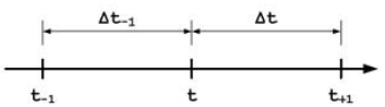
Figure 6 Vision of time in the SD simulation engine at instant t. Taken from the System Dynamics Model for the implementation of Information Technologies in University Strategic Management by Morlán (2010, p. 72).
Currently there are flexible simulation environments that allow building models in a friendly way, which automatically creates dynamic equations and simulates models in real time, showing their behavior. This research used Vensim® from Ventana Systems Inc.
3.10. Model validation
It is important to consider the difference between the concepts of verification and validation when evaluating the system dynamics model. Verification focuses on the model’s internal consistency. "The implementation of the simulation instructions to be executed on a computer is checked, i.e., whether the model has been built correctly.” In this sense, Forrester believes that: The validation or degree of significance of a model should be judged by its convenience in relation to a particular purpose. A model is logical and defensible, if it achieves what is expected of it, (...) validation as an abstract concept, divorced from its purpose, and has no useful meaning (p. 77.)
Forrester and Senge (as cited in Morlán, 2010) propose objective evalidity evidence. They emphasize that a model is built for a purpose and its validity is determined primarily by the degree in which that purpose is fulfilled. They place special emphasis on the model’s boundaries, recognizing that a model is a simplification and that the boundary between what has been included and what has not is a significant determinant of the model’s validity. As a result, they propose a series of tests of the model’s structure, the behaviour and the implications of the policy (p. 78.)
Additionally, Barlas analyzes the limitations of using statistical tests on the output of a system dynamics model and real world data. It asserts that the tests should focus on the validation of model behavior patterns rather than checking the coincidence between the actual data and that generated by the model, since, as Sterman (2000) had pointed out, a reproduction of the system's behavior, data-by-data, is virtually impossible, even if the model is structurally appropriate (p. 79.).
Also, Coyle is the one who associates the validity of a model to be well adapted to its purpose and properly built. Its main philosophy is that the model must do the same things as the real system and for the same reasons. He insists on dimensional coherence and proposes the rules for it. It underlines the need for the correspondence between the model and the problem, and that all constants must be properly defined and that their dimensions must be indicated, as Forrester had proposed (p. 79.) Tables should be integrated within the text. Please convert table files prepared in Microsoft Excel into Word format. The size of tables should not exceed the width of two columns.
4. Results
The following are the results of the research, which are initially made up by the root definition, obtained through the application of the SSM. Subsequently, the conceptual model of feedback loops obtained using the postulates of Peter Senge's systemic thinking is shown. From this model, the flow model is obtained applying SD. Finally, the model is validated with simulations carried out in the Colombian poultry sector.
4.1. Conceptual Model of Strategic Project Management for Industries (SPMI)
This part of the research covers the Conceptual Model of Strategic Management of Projects for Industries-(SPMI) aimed at the industrial sector, through the use of the causal links tool and taking into account the most important variable influencers of the Industry Project Portfolio (IPP.)
To develop the Conceptual Model, the first actions require establishing representative factors and influences on the systemic structure that are predominant. In this case, factors present in the growth of production levels from project portfolio levels in the perspective of bibliographic observation are based on this regard.
The development of the conceptual model of causal relationships eases the creation of the IPP flow model, which is necessary to test portfolios of projects and explore production level’s behavior through comparisons with different projects and portfolio levels.
4.2. Analysis of Colombia’s project planning model
Colombia’s planning at national level is executed by the National Planning Department (DNP, for its Spanish acronym.) This is an administrative unit within the executive branch of public power, directly dependent on the Presidency of the Republic. The DNP is imminently technical and its mission is fostering the implementation of a strategic vision for the country in the social, economic and environmental fields. Additionally, it designs, steers and evaluates Colombian policies by public authorities in terms of management and allocation of public investment for government plans, programs and projects.
The Colombian State allocates specific functions to government entities at different levels of planning in order to institutionalize the planning process, namely: governing entities, executing entities and approval entities.
The DNP is in charge of allocating public investment and realizing government plans, programs and projects.
The Ministry of Finance and Public Credit defines, formulates and executes policies for the country's economy, as well as related plans, programs and projects to achieve a comprehensive view of the strategic planning macroprocess of investment in project portfolios within the Colombian State.
Planning is defined in Colombia’s 1991 Political Constitution, which made it stronger and added stability. In the Constitution, structural and planning entities are in charge of the process.
Article 346 of the Political Constitution states that The National Development Plan (PND, for its Spanish acronym) is the source of expenses and that the government will annually formulate the income budget and the Appropriations Law that must correspond to the PND. This Plan is structured according to the Organic Law of the Development Plan: Law 152 1994. Table 1 describes the structures of the PND.
Table 1 Structure of the Development Plan. Built with Planning and Budget Management data. System of Planning. DNP, 2014, paragraph 70.
| General part of the plan | Investment plan |
|---|---|
| - National and sectoral objectives of the State’s mid-term and long-term action. - National and sectoral objectives of the State’s mid-term and long-term action. - Strategies and policies in the economics, social, and environmental fields. - Marking of forms, means and instruments of linking and harmonization. |
- Projection of financial resources available for execution and harmonization with public spending plans. - Description of plans and subprograms, with indication of objectives, goals and priority projects’ investment. - Multi-year budgets. |
Another important definition of the planning process in Colombia is the budget that constitutes tax policy’s quantitative expression in its intertemporal relationships, with fundamental macroeconomic relationships being the instrument that materializes State action, the Plan is executed as national development. The budgeting system comprises the Nation’s Financial Plan, Annual Budget and Annual Operational Investment Plan.
The POAI consists of investment projects classified per sector, entities and programs. It is prepared by the DNP along with the Ministry Finance and Public Credit and it is based on the Financial Plan. The POAI must be aligned with the National Investment Plan.
CONPES documents are technical instruments for coordination and planning through which the government draws economic and social policy lines.
The DNP coordinates the preparation of these documents undertaking qualitative and quantitative analysis on a specific problem and formulating actions to contribute to its solution. CONPES documents define policies’ objectives that are framed within the PND and articulate necessary interventions by entities to fulfill them.
The National Bank of National Investment Programs and Projects (BPIN, for its Spanish acronym) is a planning instrument that records viable public investment programs and projects, which have been previously evaluated considering social, technical, environmental and economic aspects and that could be financed with resources from the Nation’s General Budget.
The aforementioned references were used as observational basis to trace the root definition, necessary to start developing the IMPS Conceptual Model. The table below was constructed by analyzing each document, where each of the PQR questions is answered to construct the root definition shown in Table 2.
Table 2 PQR Formula for the Industry Project Portfolio Budget Formulation Process.
| Q What? | Q How? | A Why? |
|---|---|---|
| Manage a project portfolio that provides a quantitative positioning of the industry compared with the competition (with the average and with the best). |
Establishing best practices for standardizing project execution and helping optimize project quality, time and cost goals, and aligning them with the business plan |
To analyze the risk involved and decide to commit the necessary resources, in order to realize the idea, maximizing the chances of success |
Root definition: The Strategic Office of Project Management is responsible for receiving and reviewing strategic projects and the Project Management Office of the Industrial Sector is responsible for applying and executing resources allocated to the project groups. These activities must be carried out by actors to guarantee that the projects selected for a portfolio -in the current year- have a positive impact on the value of the business in terms of production and productivity.
The definition was constructed and it was verified using the CATWOE analysis which consists of observing if the six factors that must be explicit in any root definition are present.
The analysis of the definition described above is shown below:
P (possession): Productive sector (industries)
A (actors): Portfolio and Project Management Offices
T (transformation process) entries: projects resulting from the sector’s strategic requests
Departures: authorized projects, closed projects and deferred projects
C (consumers): operations, production and functional units
R (resources): financial, human, physical and technological resources
W (weltanschauung): improvement in production and productivity (added value to the business) and satisfaction of all stakeholders
4.3. Building the conceptual model
The model that represents causal relationships is constructed using the root definition. This construction is based on the action verbs present in the root definition, which were transformed into subsystems in order to define the "minimum necessary" activities implicit in the definition.
This second phase involved defining the causal relationships between the elements that make up the system in a causal model, hereinafter the Conceptual Model of Dynamic Interrelationship for forecasting results of planning-investment and execution of IMPS industrial projects, taking into account that it only shows causal ties and does not include other characteristics, such as information about testing time or the variables’ nature and magnitude.
Figure 7 shows the IMPS Conceptual Model presented in this article. Relationships involving some feedback loops and external source relationships are represented. The six feedback loops in which the model is structured are also displayed.
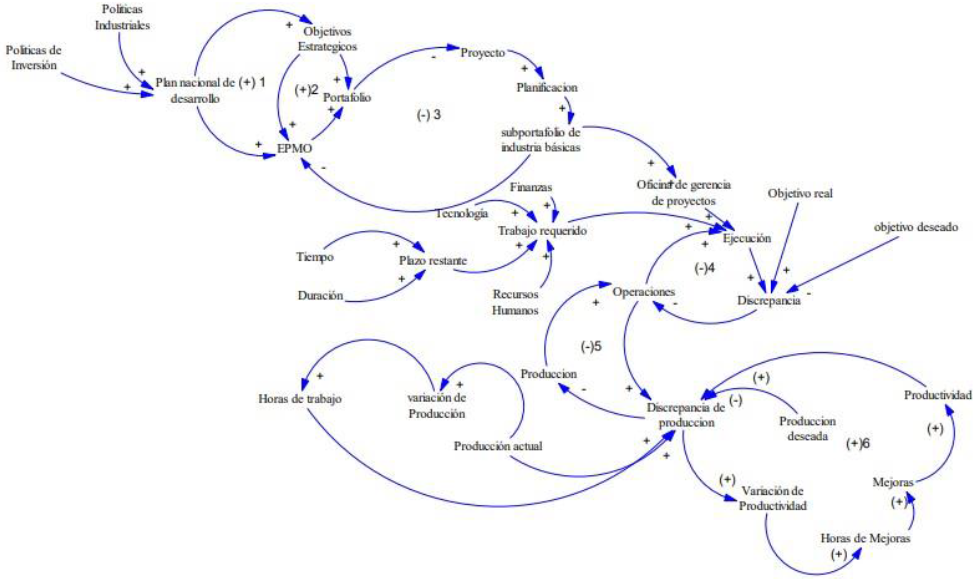
Figure 7 Strategic Project Management for Industries (IMPS) Conceptual Model. Compiled by the authors
The Conceptual Model in this article consists of six feedback loops described below:
Loop 1: Strengthening strategies of the National Development Plan or Sectoral Strategic Plan or Corporate Strategic Plan
Loop 2: Strengthening the project portfolio
Loop 3: Portfolio readjustment by project authorization in the Project Management Office (PMO)
Loop 4: Project readjustment by execution, closing or deferral
Loop 5: Readjusting by production recovery
Loop 6: Productivity boosting by operational improvements
Loops 1, 2, and 6 are positive feedback loops, i.e., they tend to destabilize system behavior and trigger system output. However, loops 3, 4, and 5 are negative feedback loops that regulate and balance the system. Finally, the model measures productivity variation, as each completed project must produce operational improvements that are represented in the latter readjustment loop.
Section 4 develops the Forrester diagram to test different scenarios and test the hypothesis raised in section 2. In this sense, modeling allows to verify the hypothesis (test variable or input) and provides a basis for designing learning laboratories that are useful for work teams in organizations.
4.4. Forrester diagram or flowchart
In order to develop the Forrester diagram or flow model, SD is used as a methodology to study and manage complex feedback systems.
This section shows the Strategic Project Management Flow Model orienting it to the industry’s sector (hereinafter identified by its acronym SPMFM), the mathematical models that gives rise to the first-order differential equations, mathematical representation and algorithms of the SD methodology and Vensim language.
4.5. SPMFM proposed in this article
The Vensim dynamic simulation software (PLE x 32 version) was used to develop the SPMFM. This program enables easy simulations of real systems’ complexity. This requires a series of symbols that allow representing particular situations and behaviors described in the methodology.
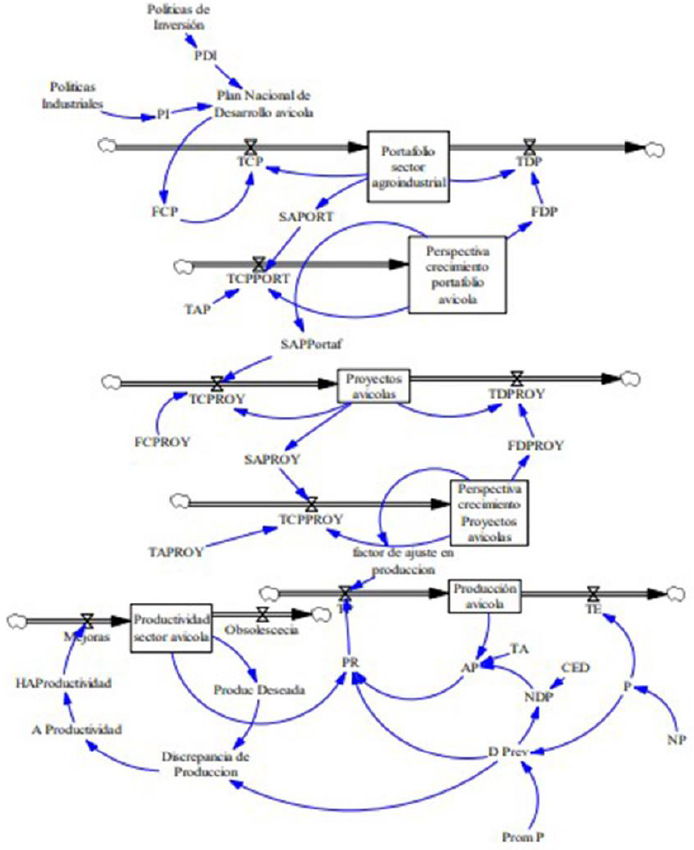
To generate the flow model, the interrelationships between the different variables that are represented in the Conceptual Model are translated into a Forrester diagram.
SPMFM’s Forrester diagram shown in Figure 8 represents a system that responds to Strategic Industrial Project Management, which begins with the positive feedback cycle. An increase in this cycle awakens a motionless negative project portfolio cycle. The negative cycle does not appear spontaneously. It is present at any time, but its size depends on the strength of the variables Industrial Policies and Investment Policies, and on which are in the positive cycle.
When the positive cycle begins to increase all the variables that appear involved in it, the negative cycle is also amplified until the domination changes and the negative cycle becomes the owner of the situation.
By assuming a portfolio in an environment with limited resources, the critical variable is the number of projects to which resources can be allocated. The number of portfolio projects increases due to the portfolio growth rate. This growth rate reinforces the positive feedback cycle. However, a negative feedback cycle is hidden. Increasing the number of projects and a fixed amount of resources causes the source of funding for each project to fall. When the amount of resources is not sufficient, some projects begin to be closed or deferred in the portfolio. The negative cycle reduces the growth rate until the amount of resources is enough to support the number of portfolio projects.
Systems that follow population growth behavior, such as project portfolio behavior, are characterized by contentions or growth limits. For projects, the limitation is the amount of resources. This contention indicates the maximum number of projects that the system can support.
Several levels and flows produce project portfolio-like behavior. Figure 8 represents a structure of the SPMFM that intuitively shows feedback cycles, the limitation of a project portfolio system in the Industries Sector and its impact on the production variable, the subject of this research.
Two feedback cycles regulate the output flow of the level. A connector binds the current value of the level to the output stream and causes a negative cycle. The second of the negative cycles passes through the portfolio's decrement factor, which is responsible for changing the dominance of the cycle. The level -initially- grows only if the portfolio growth factor is larger than the portfolio's decline factor. When the portfolio growth factor is larger than the decrease factor, the input stream is greater than the output stream and the system grows exponentially.
The level, however, cannot grow infinitely. When the level increases, it causes the level effect variable to multiply. This variable determines the effect of the level on the system rate of decrement variable. When the effect of the level takes values greater than 1, the variable rate of decrease increases. When the effect of the level increases until the variables rate of decrease and growth rate are equal, the output flow matches the input stream and stops growth. The system is in balance.
The positive flow size is not constant. Conversely, the negative cycle increases as the level increases. The output flow is the product of the level and the variable rate of decrease. Here's the key to understanding what the cycle dominates: the rate of decline increases when the level does. When this is small, the feedback cycle is negative, but when the level increases, the negative cycle increases. Finally, negative feedback leads the system to balance.
This happens with each of the four levels represented in the SPMFM (portfolio, project, production and productivity) allowing in each feedback cycle, using the mathematical logic of SD, seeing the behavior of the system when portfolio and project levels are adjusted or tested, and their impact on production and productivity, which we discuss here.
4.6. SPMFM equations
In the case of the SPMFM, equations are inferred according to the equation-based model, which is graphically represented in Figure 8. These equations in Vensim language are as follows:
Level or state equations: based on Forrester's hydrodynamic simile model
Flow or decision equations: based on Forrester's positive and negative feedback loop model.
Each of the parameters has been considered strictly greater than zero. The growth and decrease rates of each of the level variables correspond to the values to which the level or state variables are increased and decreased.
4.7. Application of the SPMFM in the agro-industrial sector - Colombia’s poultry subsector
The Colombian poultry industry was chosen to apply the model, as part of the agro-industrial sector it is considered a representative industry.
The Colombian poultry sector has been positively evolving in recent years and is one of the drivers of livestock production growth. In 2018, this industry recorded a growth rate of 4.8% which was 1.2 percentage points higher than 3.6% by 2019. For the posture sector, an increase of 5.6% was achieved when 7.1% had been planned for eggs. Moreover, the result for broiler chicken was 4.2% compared to a projection of 1.7% (Magazine of the Colombian Federation of Poultry Farmers of Colombia - (Federación Nacional de Avicultores de Colombia, 2017, p.1).
4.7.1. Scenario analysis in Colombia's poultry sector
The flow model shown below is based on the Conceptual Model of causal loops used for the SPMFM flow model, explained in section 4. This section shows the application in the agro-industrial sector, and more specifically in the poultry sector (in Colombia) by specifying two scenarios with adjustment in the time of perception of change, in the prospects for growth of portfolios and projects.
To continue the validation of the model, portfolios of projects are tested in the Colombian poultry sector of Cundinamarca changing the input parameters and adapting them to this new sector and environment.
Figure 9 presents Test 1 (P1) for the Colombian poultry sector and takes the following initial values of the decision parameters:
Agro-industrial portfolio level: 5 portfolios. Poultry projects at level: 26 projects. Poultry production level: 1,800,000 tons. Agro-industrial portfolio adjustment time: 48 months. Poultry projects adjustment time: 12 months.
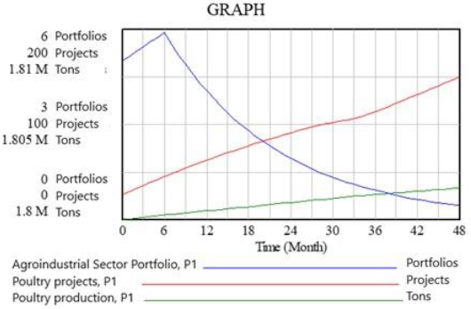
Figure 10 presents Test 2 (P2) for the Colombian poultry sector and takes the following initial values of the decision parameters: Agro-industrial portfolio level: 5 portfolios. Poultry projects at level: 26 projects. Poultry production level: 1,800,000 tons. Agro-industrial portfolio adjustment time: 24 months Poultry projects adjustment time: 6 months.
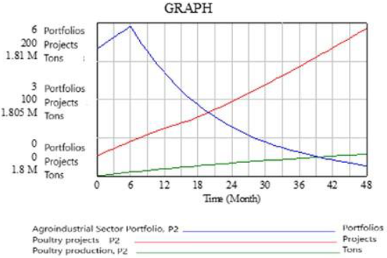
These scenarios visualize that reducing adjustment times as a key variable allows an increase in agro-industrial projects but does not sensitize production since they do not yet translate into completed projects.
Figure 11 presents Test 3 (P3) for the Colombian poultry sector and takes the following initial values of the decision parameters: Agro-industrial portfolio level: 5 portfolios. Poultry projects at level: 26 projects. Poultry production level: 1,800,000 tons. Agro-industrial portfolio adjustment time: 24 months Poultry projects adjustment time: 6 months. Production adjustment factor: Graphical function (([(0,0)-(10,10)],(0.550459,1.09649),(1.95719,3.15789),(3.82263,4.47368),(4.55657,5.13158),(5.84098,5.52632),(8.07339,6.22807) ).
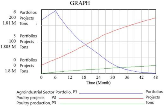
The scenario shows that the portfolio is depleted faster and poultry projects tend to stabilize to the same extent, however the increase in projects still at the end of the simulation does not substantially increase poultry production.
Figure 12 presents Test 4 (P4) for the Colombian poultry sector and takes the following initial values of the decision parameters: Agro-industrial portfolio level: 5 portfolios. Poultry projects at level: 26 projects. Poultry production level: 1,800,000 tons. Agro-industrial portfolio adjustment time: 24 months Poultry projects adjustment time: 6 months. Production adjustment factor: graphical function (([(0,0)-(10,10)],(0.550459,1.09649),(1.80428,3.46491),(2.69113,5.26316),(3.73089,7.01754),(4.95413,8.28947),(6.48318,9.3421)).
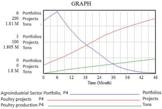
In these scenarios, maintaining the same parameters as Test 3 and adjusting the graphical function that represents the adjustment factor, leads to an increase in poultry production at the end of the 48 months of simulation.
Figure 13 presents Test 5 (P5) for the Colombian poultry sector and takes the following initial values of the decision parameters: Agro-industrial portfolio level: 5 portfolios. Poultry projects at level: 26 projects. Poultry production level: 1,800,000 tons. Agro-industrial portfolio adjustment time: 24 months Poultry projects adjustment time: 6 months. Production adjustment factor: graphical function ([(0,0)-(10,10)],(1,0.8),(1.86544,2.54386),(2.07951,3.72807),(2.47706,4.69298),(2.78287,6.09649),(3.08869,7.80702),(3.24159,9.42982) ).
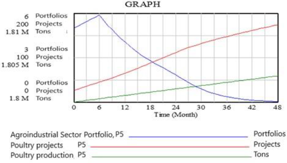
In Test 5 a greater adjustment in the production factor combined with the adjustment times of the projects, increases poultry production levels in the simulation period in the model.
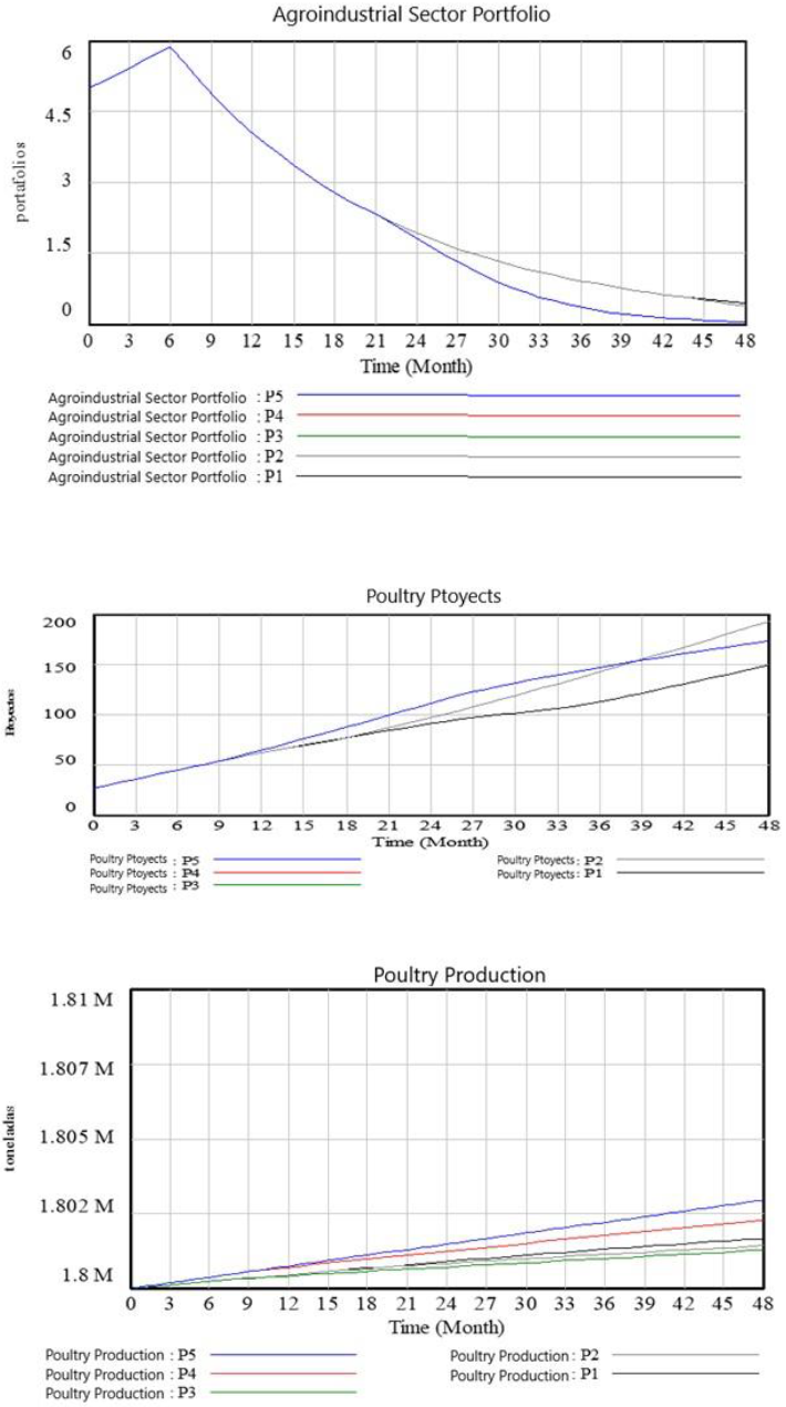
To summarize the five tests, it is possible to visualize the increases in production levels according to the parameter settings in Figure 14.
5. Discussion of Results
A different approach has been followed from that existing in the literature. It may not provide new data, nor demonstrate the existence of new variables, nor check the strength of the relationship between two variables. Instead, the main contribution of this work is obtaining new knowledge from the variables and existing relationships that had not been combined until now. This research adds value from a mathematical point of view that is different from the classic approach of Strategic Project Management.
The focus was to identify the problem by combining the root definition of SSM and SD, based on the variables and existing relationships in the literature (Project Management Institute-PMI and Axelos) and on the observation, to build a novel model that is based on equations, as opposed to a qualitative model, and that serves as a foundation for learning in decision-making when selecting projects aligned with the organizational strategy, which have an impact on operational production policies (mainly in production recovery).
The evaluation of said learning is left for future work. Likewise, an exhaustive bibliographic review of the existing models on Project Portfolio Management was compiled. Also classical approaches to strategic thinking were examined. It is an area of multidisciplinary research that encompasses the branches of strategic thinking of projects and portfolios, production and productivity, but that needs to be harmonized. With this combination of area knowledge in an integrative review and based on a dynamic model, it is confirmed that the implementation of the Management Project Strategy is a truly multidisciplinary challenge.
In addition, there is a contribution from the academic and curricular point of view. Professionals and managers in the industry sector who have to lead the decision-making processes of project portfolios need to have a broad systemic perspective, as well as robust management knowledge on strategies, projects and portfolios. And this should be extended to the study plans that certify access to industrial engineering.
The result of this research is a dynamic model, based on observations, expertise and existing theories, which represents a breakthrough in the level of specificity of the systemic relationships (from the quantitative point of view,) for the construction of prospective scenarios at industries’ strategic levels. The variables and relationships that make up the model were based on the existing bibliography and in the judgment of experts, but as a whole, it shows a new vision of the problem being studied. The proposed model shows a qualitative-quantitative behavior of the system and is a tool that helps understanding the project portfolio management process, with great impact on operational production policies, specifically in production.
The model represents a mathematical abstraction of reality that involves a loss of wealth, but that verifies the existence of two advantages: First, the simulation confirms the coherence of the assumptions derived from the theoretical framework (conceptual). Second, the model provides a virtual laboratory in which consequences of the interaction of policies’ fundamentals can be detected for investment and industrial, strategy, projects, portfolios and operational production policies.
The latter shows that dynamic simulation models can hasten the learning curve for decision makers providing a new vision of the system’s structure and its dynamic behavior. Equally, it allows them to function in different scenarios, to rehearse different policies and experience the consequences of their decisions. Altogether, it is a methodology that helps communication and discussion of the key elements of management. This demonstrates the usefulness of SD to operate complex problems for which there are no universal solutions. In conclusion, it is a tool that helps decision-making.
The contributions of this research will be used by both researchers and experts. For the academy, the product of this research offers a coherent set of theoretical references necessary for the study of Strategic Project Management. Industry professionals can use this knowledge to develop scenarios that facilitate the decision-making process at strategic levels in the industry.
The originality of this research lies in presenting a dynamic model in comparison with existing linear models. Various publications in different areas argue that the implementation of best practices or processes in Portfolio Management, strategies and projects in the theoretical investigation of this work are complex; however, they are linear. In this research the problem is approached as a complex system dynamic created from the interaction of different feedback mechanisms. The SD approach is appropriate because faced with a problem in which it is not possible to find optimal or overall solutions, there is a good opportunity to obtain trends and behaviors.
6. Conclusion
It can be concluded that the proposed Conceptual Model and the Forrester diagram help evince the dynamic interrelation of project strategy in the industries. These two models were applied to the Colombian poultry sector, and their validity was verified, however, it can be tested in other types of industries to verify its application and innovative nature. Likewise, the definition of the flow model allowed compiling a body of information related to an industry projects’ portfolio system to build scenarios and thus make decisions based on significant variables’ behavior. The flow model proposed in this document could be used to simulate the diversity of conditions. Also as a methodology for Strategic Project Management to plan scenarios that reduce uncertainty in industries’ strategic decision-making processes. In conclusion, the SPMFM proposed in this research, unlike existing linear models such as the Standard for Portfolio Management of the Project Management Institute-PMI or the Management of Portfolio of the United Kingdom (Axelos), corresponds to a model based on first-order differential equations, which allow seeing Strategic Project Management as a system and build quantitative prospective scenarios to steer the decision-making process.
Conflict of interest
The authors have no conflict of interest to declare.
Financing
The resources for this publication come from the call for co-financing of projects with external stakeholders of the Grancolombiano Polytechnic.

