SciELO - Scientific Electronic Library Online

 
vol.64 número1Refractive index evaluation of porous silicon using bragg reflectorsEffect of pressure on structural, electronic and optical properties of SrF2: a first principles study índice de autoresíndice de materiabúsqueda de artículos
Home Pagelista alfabética de revistas  

Servicios Personalizados

Revista

Articulo

Indicadores

Links relacionados

  • No hay artículos similaresSimilares en SciELO

Compartir


Revista mexicana de física

versión impresa ISSN 0035-001X

Rev. mex. fis. vol.64 no.1 México ene./feb. 2018


Research

Research in Condensed Matter

Diffusion microrheology of ferrofluids

R. Peredo-Ortíza 

M. Hernández-Contrerasa 

aDepartamento de Física, Centro de Investigación y Estudios Avanzados del Instituto Politécnico Nacional. Apartado Postal 14-740, Ciudad de México, México.


Abstract

We provide a statistical mechanics approach to study the linear microrheology of thermally equilibrated and homogeneous ferrofluids. The expressions for the elastic and loss moduli depend on the bulk microstructure of the magnetic fluid determined by the structure factor of the suspension of magnetic particles. The comparison of the predicted microrheology with computer simulations confirms that as a function of relaxation frequency of thermal fluctuations of the particle concentration both theory and simulations have the same trends. At very short frequencies the viscous modulus relates to the translational and rotational self-diffusion coefficients of a ferro-particle.

Keywords: Viscoelasticity; ferrofluids; microrheology; rheology; colloids

PACS: 83.60.Bc; 83.80.Gv; 47.65.Cb; 66.10.cg; 83.60.Df

1. Introduction

Ferrofluids are colloidal suspensions of permanently magnetized particles of nanometer size dispersed in a solvent. Their rheological properties such as viscosities, storage of energy and dissipative moduli can be controlled with external magnetic fields 1, which makes them valuable in diverse technological applications. Much of the research on these magnetic fluids relates to the class of magnetorheological suspensions which develop bulk magnetization under external magnetic field conditions 2. External fields produce chain-like aggregates of the colloidal particles, an effect that can also be developed in ferrofluids in the absence of fields for sufficiently high particle’s dipolar moment or concentration. It has been observed that when the fluid is subjected to an applied increasing shear rate they change from their Non-Newtonian (nonlinear relationship of stress with the applied shear flow, which it can be produced by thermal fluctuations too) to Newtonian (the stress response of the liquid is linear through a kernel with the shear rate. With the kernel been the stress relaxation modulus) under magnetic fields. Such rheological behavior has been demonstrated to be anisotropic through the use of macroscopic rheology experiments 3, and also more recently through a no invasive technique, the passive microrheology on a probe particle diffusing in the colloidal suspension 4 in thermal equilibrium. In their development of this latter experimental technique by Mason et al5, they express “bulk relaxations have the same spectrum as the microscopic stress relaxations affecting the suspended particle motion". They assumed that the complex shear moduli can be determined from the particle’s mean squared displacement in the linear regime of low shear flow. This technique has a significant sensitivity and detects high frequencies of relaxations as compared to macroscopic rheology. Ferrofluids look dark with visible light because of its strong absorption by the ferro-colloids. Mertelj et al.4 were able to measure the translational diffusion of the probe particle with their use of low-intensity laser beams in dynamic light scattering experiments. In their research, they used small samples which together a careful selection of wavelengths allowed them to reduce the absorption of light by the ferrocolloids. Whereas Yendeti et al6 made their microrheology experiments observing a fluorescence silica colloidal particles suspended in the ferrofluid. This way they were able to use video microscopy to track the silica particle positions driven by its Brownian motion inside the ferrofluid. Thus, fine tuning of the wavelength to the order of the probe particle size allows the determination of its mean squared displacement. Therefore, the scattered light originates only from the probe silica colloidal particle since the molecules of the solvent are much smaller than the wavelength of the used light. Solvent provides the reservoir that dissipates energy from the translational and rotational movement imparted by the Brownian motion of all the colloidal particles. It was shown in Refs. 7 and 8 that dynamic light scattering and video microscopy in microrheology experiments allows the determination of the orientation variable, thus, providing the rotational diffusion of the probe. From its angular displacements, the time-dependent mean squared angular displacement was measured. Consequently, the microrheological shear modulus of the host suspension was obtained. Comprehensive theoretical knowledge of the main measured rheological properties have been reached with thermodynamic 9,10,11,12,13,14,15, and kinetic theories of liquid crystal dynamics 16 that involve macroscopic constitutive magnetization’s relaxation mechanisms, and both mean field and microscopic free energies of the thermodynamic state, respectively. Thus, the experimentally observed dependence of viscosity with magnetic field was accurately confirmed with a kinetic approach from low up to moderate concentrations before the formation of chain structures by the particles 17. After the formation of chains, a so-called kinetic chain theory of rod-like aggregates 18,19 confirms the observations on the increase of viscosity with field quantitatively. In a similar set of macroscopic experiments at low strain in a system where the finite size of the vessel containing the liquid was important 20, it was determined the energy dissipated due to aggregate’s structural deformation when they are partially bound to the confining walls. It was found that the aggregates experience cohesion and movement of their inner constituting particles which generates heat through this process. Such a heating mechanism is relevant in hyperthermia applications where ferro-particles diffuse, rotate and stick to the boundaries in the multicomponent medium inside of a tissue 21. These findings have raised the interest to investigate the rheology of complex fluids of mixtures of added polymer solutions to the magnetorheological fluid 20,22,23,24. Thus, the theoretical description of their observed rheology and effect of size polydispersity 25,26,27,28, have been described with polymers motivated models 29,30. More recently, theories based on macroscopic thermodynamics predict as in polymer theory elongational viscosity and its consequence on the ratios of the viscoelastic moduli 30, and of the module to viscous dissipation time. Such predictions were adopted in the microrheology experiments of Refs. 4,6 in order to get estimates for the values of all anisotropic properties. In the present manuscript we propose expressions for the complex shear modulus response for the rheology of an equilibrium ferrofluid derived from a statistical mechanics approach valid in the regime of linear shear flow of microrheology experiments. The viscoelastic moduli depend on the pair distribution function which captures the bulk microstructure of the ferro-particles due to their pair direct interactions. We show that for a given concentration of particles, ferrofluids at equilibrium state display rheological behavior in a similar way as it is observed to occur in non-equilibrium anisotropic magnetic fluids under external fields and shear flow. For the dispersed homogeneous phase of the colloid, we found that the dissipative modulus is dominant at low frequencies where the colloid displays a liquid character with a crossover to an elastic fluid mode at moderate frequencies where the elastic modulus becomes dominant at higher frequencies. The calculated loss modulus has good agreement with Langevin dynamic simulations up to the transition to the elastic behavior where it starts to deviate. Whereas the general shape of the elastic modulus, as obtained from simulations of the mean square translational displacement of a probe ferro-particle is qualitatively well described by the model proposed. An increase of the dipolar moment per particle or of their concentration can lead to the formation of chain like aggregates in absence of external fields. Our model theory of microrheology is useful in this case too. Since the formation of chains is taken into account properly by the pair correlation function which describes the bulk micro-structural order of the particles due to their direct interactions. We also provide the analytical expressions for these moduli when the observable is the mean square angular rotation for experiments that observe the rotational diffusion of ferro-particles. These viscoelastic properties can also be used to study in the linear regime of flow the rheology of equilibrium isotropic ferroelectric colloids 31,32,33.

2. Translational diffusion microrheology

Tracking microrheology experiments are useful techniques that accurately provide the linear viscoelasticity of suspensions of polystyrene particles and other complex fluids 5,7,34,35. In these experiments it is assumed that the complex shear moduli can be determined from the particle’s mean squared displacement in the linear regime of low shear flow. The rheological properties are extracted through the equilibrium Einstein expression of the friction on a probe particle that performs a Brownian motion in the colloid. The friction due to interaction with its neighbors, in the frequency space ζ(ω), that affects its translational movement is related to the mean square displacement <Δω(ω)2> and to the complex shear modulus by

G(w)=kBTiπa<Δr(ω)2>=iω(ζ0+ζ(ω))3πd (1)

with i=-1. a the particle radius. ζ0 the solvent friction on a particle. In what follows we show how the friction on the probe particle is obtained.

The Langevin equations of the translational and rotational Brownian motion of the probe particle that interacts with the others in the suspension are the stochastic Eqs. 36

MdVtdt=-ζ0Vt-ζTR0Wt+f0t+FTOTt IdWtdt=-ζR0Wt-ζRT0Vt+t0t+TTOTt (2)

V(t) and W(t) are the translational and angular velocities of the probe. We used a space fixed frame with origin at the particle center of mass, and frame axis following the orientation of the probe main axis of symmetry. M and I are the mass and particle’s matrix of moment of inertia, respectively. We shall not consider neither hydrodynamic interactions among particles nor external magnetic fields. The first two terms in Eqs. (2) are the solvent friction force and torque. The short time free particle diagonal friction tensors ζ0, ζTR0, ζRT0, ζTR0, ζRT0 represent hydrodynamic drag forces, and torques. These friction and random forces are the only quantities that convey information on the nature of the solvent. And they ignore their molecular degrees of freedom of position and orientation coordinates and momenta. They are coupled to the thermally driven solvent random forces f0 and torques t0 by the fluctuation-dissipation theorems

f0(t)f0(0)=kBTζ02δt,                      f0(t)t0(0)=kBTζTR02δ(t),t0(t)f0(0)=kBTζRT02δ(t),                     t0(t)t0(0)=kBTζR02δ(t) (3)

and kB Boltzmann constant, T = 300K the absolute temperature. The total force FTOT and torque TTOT on the probe by the other colloidal particles which are at the concentration n(r,Ω,t)=i=1Nδ(r-ri(t))δ(Ω-Ωi(t)) are given by

FTOTt=drdΩψr, Ω nr, Ω, t,       TTOTt= drdΩr×ψr, Ω+Ωψr, Ω n r, Ω, t (4)

with Ω=(θ,φ) and θ,φ being the polar angles, ψ(r,Ω,Ω') is the pair potential, and Ω=n^×n^ the angular gradient operator. It should be noted that FTOT (t) and TTOT (t) are calculated using the probe’s dipole located along the Z axis direction of the its local frame, that is Ω'=(0,0). The unitary cartesian vector n^ of the orientation of any other particle is in the direction of that particle’s axis of symmetry.

Both Langevin equations can be written compactly as

MdV(t)dt=-ζ0V(t)+f0(t)+drdΩψr,Ω n(r,Ω;t), (5)

where =(,r×+u×d/du) is the general gradient operator. r denotes the vector joining the centers of the probe and another particle. u is a unitary vector with orientation θ,ϕ. The generalized velocity V=V,W, Mij=Mδij (i,j=1,2,3),Mij=δijIi-3 (i, j = 4,5,6), with I 1, I 2, I 3 being the principal moments of inertia of the tracer. The friction tensor ζ0 is a diagonal matrix which have the nonzero components with elements ζ110=ζ220=ζ0, ζ330=ζ0, ζ440=ζ550=ζR0, and ζ660=0 which are external inputs to this theory and are provided by experiment or an external theory. For spherical particles ζ0=ζ0=ζ0. Such coefficients describe the particle hydrodynamic friction with the solvent when its diffusion occurs along its dipole orientation (), perpendicular (), or performs rotational motion R. Equation (5) can be written to first order in concentration fluctuations δn(r,Ω;t)=n(r,Ω;t)-neq(r,Ω), with the profile distribution of host particles in the probe’s field given as neq(r,Ω)=n(r,Ω,t) been an equilibrium ensemble average. Thus, the Langevin equation takes on the final form

MdV(t)dt=-ζ0V(t)+f0(t)+drdΩ[ψr,Ω]δn(r,Ω;t), (6)

where neq(r,Ω) does not contribute to the total force and torque. Similarly, a stochastic evolution equation for δn(t) is derived with help of linear irreversible theory of fluctuations 37

δn(r,Ω,t)t=[neqr,Ω]V(t)-0tdt'dr'dΩ'dr''dΩ''L(r,r',Ω,Ω';t-t')×σ-1(r',r'',Ω',Ω'')δn(r'',Ω'';t')+j(r,Ω;t), (7)

with j(r,Ω;t)j(r',Ω';0)L(r,r',Ω,Ω';t), and j(t) been a random diffusive flux. This is the more general form of the diffusion equation of the particles. Its solution is

δn(r,Ω,t)=dr'dΩ'χ(r',Ω';t)δn(r,Ω;0)+0tdt'dr'dΩ'χ(r,r',Ω,Ω';t-t')×[neqr',Ω']V(t')+0tdt'dr'dΩ'χ(r,r',Ω,Ω';t-t')×[-'jr',Ω';t']. (8)

The diffusion relaxation of the host particles around the probe is provided by χ(t) that fullfils

χ(r,r',Ω,Ω';t)t=-0tdt'dr'dΩ'dr''dΩ''dr'''dΩ'''L(r,r',Ω,Ω';t-t')×σ-1(r',r'',Ω',Ω'')χ(r'',r''',Ω'',Ω''';t), (9)

which has initial condition χ(r,r',Ω,Ω';t=0)=δ(r-r')δ(Ω-Ω'). Equation (9) can be converted into a dynamical equation for the Van Hove function of fluctuations in the concentration of particles C(r,r',Ω,Ω';t) with respect to its equilibrium value

neq(r,Ω):C(r,r',Ω,Ω';t)=dr''dΩ''χ(r,r'',Ω,Ω'';t)''

×σ(r'',r',Ω'',Ω')δn(r',Ω';0)δn(r',Ω';t),

which determines the relaxation modes of the cage of particles surrounding the probe. Its initial condition σ=Ct=0=δn(0)δn(0) is the inhomogeneous static correlation function with inverse given by

dr''dΩ''σr, r'', Ω, Ω''''σ-1r'', r', Ω'', Ω'=δr-r'δΩ-Ω' (10)

Substituting the above solution for δn(t) into the Langevin equation (6) leads to

Md(t)dt=-ζ0V(t)+f0(t)-0tdt'Δζ(t-t')V(t')+F(t), (11)

where

Ft=+drdΩψr, Ω×dr'dΩ'Xr', Ω';tδnr', Ω';0+dr'dΩ'Xr, r',Ω,Ω';t×-'jr', Ω';t' (12)

is a fluctuating generalized force arising from the spontaneous departures from zero of the net direct forces exerted by the other particles on the tracer. It groups a random force and torque on the tracer with zero mean value, and time dependent correlation function given by F(t)F(0)=kBTΔζ(t), and the time-dependent friction function on the probe (tracer) particle is

Δζ(t)=-1Ω2drdr'dΩdΩ'[ψr,Ω]×χr,r',Ω,Ω';t['neq(r',Ω')]. (13)

Using the Wertheim-Lovett’s relation 38

ψr, Ω=-kBTdr''dΩ''σ-1r, r'', Ω, Ω''×''neqr'', Ω'', (14)

we derive other useful forms of the friction function Δζ(t) as

ζ(t)=kBTΩ2drdr'dr''dΩdΩ'dΩ''[neqr,Ω]×σ-1(r,r',Ω,Ω')χ(r',r'',Ω',Ω'';t)×[''neq(r'',Ω'')]=βΩ2drdr'dΩdΩ'[ψr,Ω]×Cr,r',Ω,Ω';t['ψ(r',Ω')], (15)

with β=1/kBT and C=χσ , drdΩ, and is transpose. The angular average in (15) (division by Ω2) is necessary since this is an experimental observable. In Eq. (15) neither hydrodynamic interactions nor external magnetic fields were included. It can also be extended to describe mixtures of species of anisotropic particles with axial symmetry.

The time-dependent memory function Δζ(t) contains the dissipative friction effects derived from the direct interactions of the probe particle with the particles around it. This memory function defines the relaxation time τIτB(τB) which is the relaxation time of the momenta of the particles) for the particles to diffuse a mean distance among them. Thus, in the diffusive regime tτB, long time overdamped regime means tτI. At this time scale the momenta of the colloidal particles have already relaxed and the only relevant dynamic variables are their positions and orientations (r(t),Ω(t)).

This is a general expression for the friction contribution on the tracer due to direct interactions with the particles about it. It depends on the microstructural inhomogeneous total correlation function h(r,Ω)=neq(r,Ω)/ρ-1 of the host suspension of N particles at concentration ρ around the field of the probe, and of the free friction constants ζ0 through χ(t). We now introduce the homogeneity approximation which amounts to ignore the tracer’s field on the properties σ, χ(t) or equivalently on C(t), which then can be determined in the bulk solution. Thus, σ(r,r',Ω,Ω')σ(r=r-r',Ω,Ω',Ωr-r'). It is also adopted the Fick's diffusion approximation for χ(t)=exp(-tLσ-1), with L(r-r',Ω,Ω',Ωr-r')=ρ[D*02+DR*0Ω2]δ(r-r')δ(Ω-Ω'). In this approximation D*0=D0+Dother0, DR*0=DR0+DR,other0, (The case Dγ,other0Dγ0, γ=, , R was made in 36). The short-time diffusion coefficients Dother0=D0,DR,other0=DR0 of the other particles are approximated by those of the tracer, and D0=kBTζ0,DR0=kBT/ζR0. For spherical solid particles, ζ0=3πηsold,ηsol is the viscosity of the pure solvent, d is the diameter of the Brownian particle, and ζR0=πηsold3.

Using the above approximation for χ(t) and C=χσ, Eq. (9) can be written as

C(r,Ω,Ω',Ωr;t)t=-ρ[D*02+DR*0Ω2]×dt'dr''dΩ''σ-1(r-r'',Ω,Ω'',Ωr-r'')×C(r''-r',Ω'',Ω',Ωr''-r';t-t'). (16)

This last equation governs the diffusive relaxation of C(t), as described from the tracer’s reference frame. In this manner, we have obtained a closed approximate expression for Δζ(t) in terms only of the static properties ψ, σ and of the phenomenological quantities D0 and DR0.

From (15) the 6x6 diagonal friction matrix, where it is ignored translational and rotational coupling is

ζ(t)=1Ω2βψCt[ψ], (17)

with Ω=4π. In this theory the orientation of the probe particle’s main axis of symmetry was defined with respect to its body fixed frame. It has its dipole oriented along the main shaft u = (0, 0, 1). Thus, another particle’s orientation u=u(Ω) is denoted in this frame by the polar angles of its orientation Ωj=(θj,ϕj) for j = 1,…, N.

Thus, the friction matrix (17) has only five non zero diagonal elements; ζ11(t)=ζ22(t)=ζ(t) is the friction on the tracer for perpendicular motion to the dipole or of its anisotropy vector of orientation. ζ33(t)=ζ(t) describes the parallel motion along the main axis of symmetry. The contribution to the rotational friction is ζ44(t)=ζ55(t)=ζR(t). In Eq. (17) β=1/kBT. The general expressions for the friction function in (17) can be used also to study tracer diffusion on rod-shaped particles suspensions 39 such as fd viruses on which the experimental techniques of birefringence 40, and forced Rayleigh scattering measure the diffusion properties 41. On the other hand, the propagator in (17) C(t):=δn(t)δn(0) governs the collective relaxation of the particle’s configuration variables (r(t),Ω(t)) due to thermal fluctuations in their local concentration δn(r,Ω,t)=n(r,Ω,t)-neq(r,Ω) about the equilibrium neq=n(r,Ω,t) of its local instantaneous value n(t)=i=1Nδ(r-ri(t))δ(u-ui(t)) 38. It has initial condition C(t=0)=ρS(r,Ω;r',Ω'):=δn(r,Ω;0)δn(r',Ω';0) where S is the structure factor of particles with numerical density ρ=N/V. The temporal evolution of C(t) is given by Fick’s diffusion law which amounts to an exponential relaxation time and thus corresponds to a Maxwell viscoelastic model.

The colloidal ferrofluid is contained in a volume V. It consist of a carrier fluid which molecular nature is not taken into account, plus the monodisperse system of N spherical particles where each one has a permanent dipolar moment μ.ψij is the direct pairwise interaction potential energy between particles i, j. Because ferro-particles can not overlap their interaction is modeled by a Lennard-Jones (LJ) short range (sr) repulsive, and long-range dipolar (d) potentials ψ12=usr+ϕd

usr=4ϵ0dr12-dr6,r<2.5d (18)

with ϵ the strength, and the dipolar part

ϕd=-μ04πμ2r3D(Ω1,Ω2,Ωr). (19)

μ0 is the magnetic permeability of vacuum. D(Ω1,Ω2,Ωr):=3(r^12u1)(r^12u2)-(u1u2), where r^=r/r a unitary vector with orientation Ωr. Due to the spatial symmetry of the dipolar potential the pair correlation function g(r,Ω1,Ω2) has the fixed space rotational invariant expansion of Wertheim in the form 38

g(r,Ω1,Ω2)=g(r)+h(r)+hD(r)D, (20)

with :=u1u2.D(Ω1,Ω2,Ωr):=3(r^12u1)(r^12u2)-(u1u2), where r^=r/r a unitary vector with orientation Ωr. u is a unitary vector with orientation u=u(θ,ϕ). Another equivalent laboratory rotational invariant expansion for g(r,Ω1,Ω2) was given by Blum 38

fr, Ω, Ω'=4π32mnlfmnlr2l+1 ×μvλmμnvlλ×YmμΩYnvΩ'YlλΩr (21)

with the identification g000:=gr, h110:=-h(r)/(3), and h112:=hD(r)(10/3) dictated by the symmetry of the dipolar fluid.

By taking the Fourier-Bessel

fmnl(k)=4πil0r2jl(kr)fmnl(r)dr

42 with jl being the spherical Bessel function, and Laplace transform

C,αmnl(k,w)=0dteiwtC,αmnl(k,t)

of (16) (See Ref. 36) we find

[-iwC,αmn(k,w)-C,αmn(k,w=0)]=-ρ4πΩ(2l+1)[D*0k2+DR*0mm+1]×n1(-1)αC,αn1n(k,w)[σ-1],αmn1, (22)

where i=(-1) and

C,αmnl(k,w)=l=|m-n|m+nmnlα-α0Cmnl(k,w)

42. Using the above values of mnl = 000, 110, 112, then for dipolar liquids α=0,±1, and using the approximation D*0=2D0, DR*0=2DR0, 36 we get for (22)

C,α11(k,w)=[σ(k)],α11-iw+ρ(-1)α(D*0k2+2DR*0)[σ(k)],α11. (23)

And the inverse relation holds 42

Cmnlk, w=2l+1×α=-inf m, ninfm, nmnlα-α0C,αmnlk,w  (24)

Thus

C000(k,w)=C,000(k,w)C110(k,w)=1(3)[2C,111k,w-C,011k,w]C112(k,w)=10(30)[C,111k,w+C,011k,w]. (25)

The structure factor S=σ/ρ and total correlation function h are related by

σ,αmn(k)=ρS,αmn(k)=ρ[1+(-1)αh,αmnk], (26)

S,000(k)=1+ρ*h000(k)S,011(k)=1-ρ*d31(3)h110(k)-2(30)h112S,±111(k)=1-ρ*d31(3)h110(k)+1(30)h112. (27)

Using the invariant spherical harmonic expansion in Eq. (17) we obtain the friction function on the probe (tracer) particle

ζ(t*)=ζ012π2t0ρ*0dxx4(S,000(x)-1)2S,000(x)e-x2t*2(1+1/S,000(x))+4(3)ζ0ρ*μ*4t00dxj2(x)2{-C110(x,t*)+2(10)25C112(x,t*)}, (28)

with the single time dependent relaxation function Cα11(x,t*)=ρSα11(x)e-t*(x2+3/2)/Sα11(x), α=0,1 36. The first term on the right hand side of (28) was first derived by Nägele et al43 for spherically symmetric interacting particles and the second term in the present manuscript.

3. Microrheology under linear shear flow and no external magnetic field

We assume now that the viscoelastic response of the ferrofluid to variations of strain rate γ˙(t) is given by a linear constitutive equation for the shear stress 5

σ(t)=0tdt'G(t-t')γ˙(t), (29)

with shear relaxation modulus G(t). Because the shear stress divided by the shear rate has dimensions of viscosity, it is defined the complex viscosity η(t)=G(t)/γ˙(t). In frequency space, ω, σ(ω)=G(ω)iωγ(ω). Mason and Weitz 5 proposed that the bulk stress temporal relaxation scale of G(t) is the same time scale response as the microscopic stress relaxation of the complex viscosity η(t) that affects the particle motion. Thus for spherical particles undergoing translational diffusion they found G(ω)=iωη(ω)=ζ(ω)/(3πd) 5, whereas for rotational Brownian movement G(ω)=ζR(ω)/(πd3) 34. This approximations has resulted in a very useful experimental technique called microrheology. Thus, here we make the same approximations of Mason and Weitz in order to obtain, in the case of translational movement, the linear relationships for the rheology of the ferrofluid and described by the complex frequency ω dependent shear modulus

Gω=G'ω+ı G''ω=iωζ0+ζω3πd=iωηω (30)

where ı=(-1), ζω : =Reζω-ıIm ζω, with Re, Im the real and imaginary parts of the friction function given by the average ζ(t)=(1/3)(2ζ(t)+ζ(t)). Using the Laplace transform

f(w)=0dte-ıωtf(t)

we find

ζ(ω)=0dte-ıωtζ(t)=0dtcos(ωt)ζ(t)-ı0dtsin(ωt)ζ(t)ReΔζ(ω)-ıImΔζ(ω). (31)

Because for dipolar particles ζ(t)=(4/3)ζ(t) 36, then from Eq. (28) we determined ζ(t) from these contributions as the real and imaginary parts of the complex friction function given by (31)

The complex viscosity of a viscoelastic fluid is defined as η=η'-iη, with components η'=G/ω, η=G'/ω. Using (30) and (31) we find that

G'(ω)=ωη(ω)=ω*3πβd3ImΔζ(ω*)ζ0G(ω)=ωη'(ω)=ω*3πβd3ReΔζ(ω*)ζ0. (32)

The normalized frequency ω*=ωt0 where the Brownian time t0=d2/D0 for a particle to diffuse its diameter. The short time particle diffusion coefficient D0=kBT/ζ0 and the friction ζ0=3πηsold with ηsol the solvent (sol) viscosity. These equations are valid for a concentrated ferrofluid under a stationary shear flow. They constitute the main results of this manuscript. Finally the storage modulus is

G'ω=2ω*kBT3πd3ζ0Imζω*,  Imζω*=ω*ζ03π2ρ*0dxS,000x-12S,000x2ω*x22+S,000x+1S,000x2     +8ζ0ρ*μ*2ω*90dxj2x2       ×-6S,111x3/2+x2S,111x2+ω*2 +9S,011x3/2+x2S,011x2+ω*2 (33)

and the dissipative modulus

G''ω=ω*3πβd3+2ω*kBT3πd3ζ0Reζω*,  Reζω*=ζ06π2ρ*0dxx2×S,000x-12S,000x+1S,000x22ω*x22+S,000x+1S,000x2+8ζ0ρ*μ*290dxj2x2×6S,111x23/2+x2+S,111x2ω*23/2+x2 +9S,011x23/2+x2+S,011x2ω*23/2+x2 (34)

with h000=g000-1. For a hard ferrofluid suspension, the obtained expression of the complex modulus can be rewritten as

G'(ω)=0dxP000(x)(ω*τs,iso*)21+(ω*τs,iso*)2+0dx[P111(x)(ω*τs,1*)21+(ω*τs,1*)2+P011(x)(ω*τs,0*)21+(ω*τs,0*)2], (35)

where we introduced the auxiliary definitions

P000(x)=118π3βd3ρ*x4(S,000(x)-1)2S,000(x)P111(x)=-32ρ*μ*49πd3βj2(x)2S,111(x),P011(x)=48ρ*μ*49πd3βj2(x)2S,011(x). (36)

The imaginary part is

G(ω)=ω*3πβd3+0dxP000(x)ω*τs,iso*1+(ω*τs,iso*)2+0dx[-P111xω*τs,1*1+(ω*τs,1*)2+P011xω*τs,0*1+(ω*τs,0*)2]. (37)

Given the known material values of d,μ,ρ,ηsol,T for a ferrofluid, Eqs. (35-37) do not depend on adjustable parameters. The dimensionless quantities τs,α*=τs,α/t0=S,α11(x)/[8πx2+6] are short (s) relaxation times associated to the ferrofluid’s fluctuation in concentration in transversal (α=1) and longitudinal (α=0) modes to the wave vector. And τs,iso*=τs,iso/t0=1/[x21+1S,000x] arising from the isotropic (iso) interaction of particles. In Eqs. (35) and (37) the first and second terms arise respectively from the radially symmetric part of the potential (either this been LJ, Yukawa or hardcore type) 36,43. The second term comes from the dipolar interaction derived in this manuscript. The above equations show that there are three temporal relaxation times of fluctuations in concentration. j2(x) is the spherical Bessel function of order 2. μ*2=μ0βμ2/(4πd3), x = kd, k is the wave number. The reduced density ρ*=ρd3 and the projections of isotropic, longitudinal and transversal structure factor to the wave vector, are respectively

S,000(x)=1+ρ*d3h000(x)S,011(x)=1+ρ*3d3h(x)+2hD(x)S,111(x)=1+ρ*3d3h(x)-hD(x). (38)

The Fourier-Bessel transform of the projections of the total correlation function h000:=g(r)-1, h(r), and hD(r) were calculated according to the method of Ref. 42. These structural information results from the equilibrium position and orientation of the particles and they are determined from Brownian dynamic simulations performed with the Lammps package 44, which allows the calculation of the averages

gr=i,jijδr-rijN4πρ*r2,hr=3i,jijδr-rijuiujN4πρ*r2,hDr=32×i,jijδr-rij3uir^ijujr^ij-uiujN4πρ*r2. (39)

In Lammps simulations we used dimensionless units for, the particle energy at room temperature, length and mass which were obtained with respect to those of the ferrofluid Fe2O3, given by the values 2; ϵ0=5.453110-21J, d = 10-8 m, and m 0 = 2.70710-21 Kg, respectively. They are related by the time scale t'=dm0/ϵ0 that measures the step size in the simulations.

Figure 1 is a log-log plot that depicts the behavior of τs,α,iso* versus reduced wavenumber x for a system with dipole moment μ*=1, and density ρ*=0.3. This figure shows that τs,iso*>τs,1*τs,0*, that is, isotropic fluctuations of concentration decay more slowly than longitudinal ones. Thus, transversal modes (τs,1-1) decay more slowly than longitudinal ones. This phenomenon has also been observed by other authors in ferrofluids and dipolar colloids 46,47. In the long wave length limit kd1, it results τs,α=t0S,α11(x)/48π, which yields a relationship between the Brownian time t0 and the microscopic time τs,α. A similar relationship between the Brownian and microscopic times, through colloid microstructure, was found by Bagchi et al47. Figure 1 also implies that the short time τ,000 governing the collective isotropic density fluctuations has a larger contribution in both moduli than the longitudinal and transversal modes.

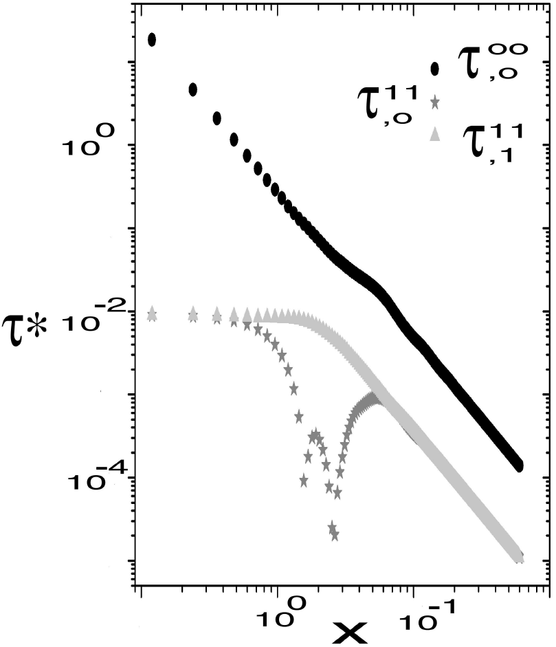
Figure 1. The viscoelastic model of Eqs. (5-8) has three characteristic relaxation times τs,α*= τs,α/t0,α=iso, 1, 0 whose logarithmic plots are provided here versus dimensionless wave number x = kd. Dipolar strength is μ*2=1 and reduced density ρ*=0.3. Transversal mode relaxation time τ,111 , longitudinal τ,011, and isotropic one τ,000 for polarization fluctuations with respect to wave vector. 

4. Viscoelastic moduli

In Fig. 2 are plotted in log-log scale the elastic G´(w) and dissipative G”(w) modulus versus frequency at three reduced densities ρ*=0.9(a),0.5(b),0.3(c) and fixed dipolar strength μ*=1.0. Notice that due to the used Lammps system of units, in the plots of Fig. 2 and further, μ*2 is replaced by μ*2/T* in all our equations leading to all figures presented below. Here kBT*=0.759559ϵ0. The simulation results for G” and G´ are depicted in black filled circle and black star symbol , respectively. These properties were obtained following the method of Mason et al.5 which require the use of the simulation or experimental results of the mean squared displacement in Eq. (1). Whereas, the theoretical predictions of Eqs. (35-37) for these properties are given in gray void star symbol for G”, and gray void circle for G´. We can observe that the model predictions of Eqs. (35-37) for both properties are in qualitative agreement with the simulation results from low concentrations up to the crossover region where the elastic response of the ferrofluid overwhelms the viscous modulus and dominates at high frequencies. After this transition region, and for the highest concentration ρ*=0.9. Figure 2(a), the elastic modulus disagree with the simulated value at all frequencies. However, there remains good agreement for the viscous modulus from low up to the crossover region. We note that whether this system presents a partial aggregation of particles such as chains or not Eqs. (35-37) are generally valid. In our model system where there are no chains. In general, the theoretical predictions for the viscoelastic moduli yield the same trends observed for these properties as obtained from simulations. At low frequencies (long times) the ferrofluid is viscous, and at the short time it is an elastic medium.

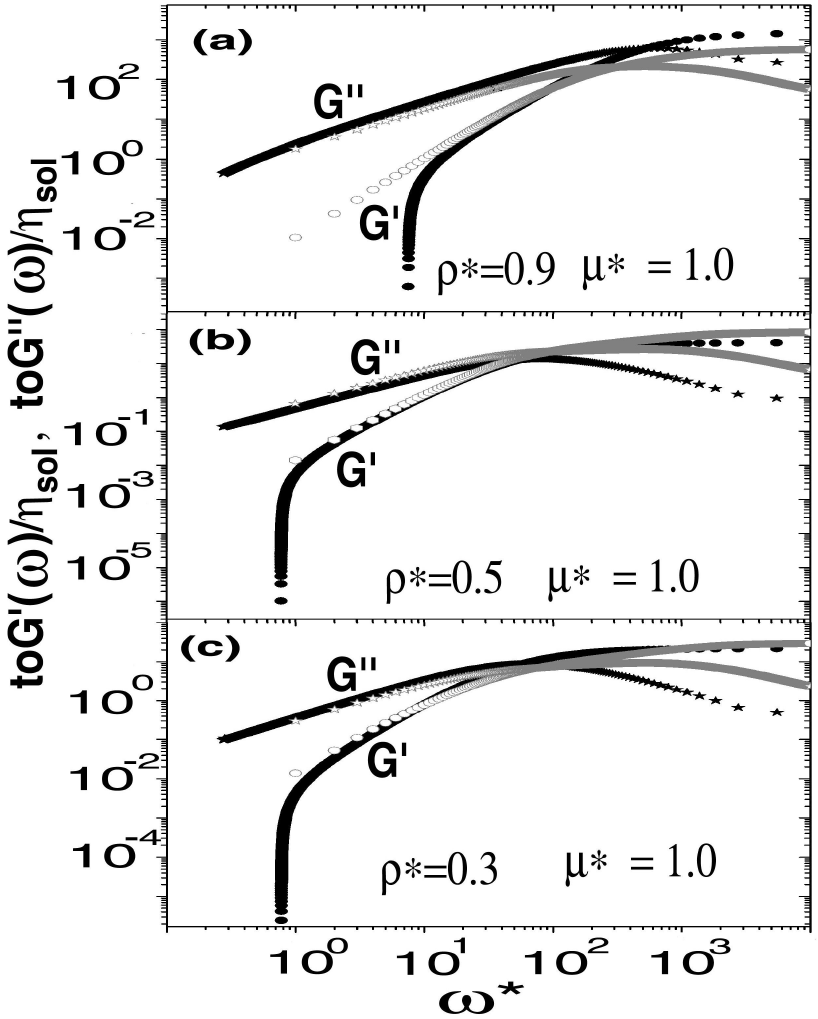
Figure 2. Logarithmic plot of elastic G' and loss G'' moduli versus logarithm of dimensionless frequency ω*=ωt0 at three different concentrations and fixed dipolar moment. Theory for G' is denoted with symbol and simulation with . Theory result of G'' is denoted by gray open star and simulation by

Our derived expressions of Eqs. (35-37) have the same frequency dependence as a continuous mechanical (mec) model of Maxwell viscoelasticity given by 45 G'=G0mec(ωτR)2/[1+(ωτR)2], G=G0mecωτR/[1+(ωτR)2] with a single relaxation time τR for magnetization relaxation. A fit of these relationships to our simulations of G', G'' is given for instance in Fig. 3 for a ferrofluid with concentration ρ*=0.1, and dipolar strength μ*=1.6. From this plot we obtained the parameters of Table I at various thermodynamic states.

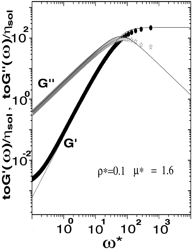
Figure 3. Brownian dynamic simulations of viscoelastic moduli as a function of frequency for a fixed concentration and dipolar moment. Simulation calculation of G' is denoted with
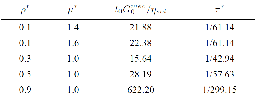
 and the continuous line attached to it is the fit with the mechanical Maxwell continuous model. Similar description for the loss modulus G''

Table I. Parameters of mechanical Maxwell model 

The value of τ*=1/ω* is were G' = G''. In Fig. 3 we provide the adjustment of such continuous model. Table 1 yields the values of the storage modulus expressed as t0G0mec/ηsol, and τ*=τR/t0 after a fitting to our simulations for G' (symbol ), G'' (symbol void gray ). In this figure, continuous line is the above macroscopic model for G', G''. In the continuous mechanical model the magnitude of the complex viscosity is |ηmec(w)|=η0/1+(ω*τ*)2 with η0=t0G0mecτ*. On the other hand, the magnitude of the complex viscoelastic modulus that follows from the statistical microscopic model of Eqs. (35-37), is |η(ω*)|=|ζ(ω*)|/3πd=t0G'2(ω)+G2(ω)/ω* which at zero frequency yields the static effective viscosity η0=t0G0, where the storage modulus of the ferrofluid is given by

G0=13πd3βζ(ω=0)ζ0. (40)

At longtimes, the self-diffusion of a particle is D=kBT/ReΔζ(ω=0)=D0/[1+ReΔζLJ+ReΔζdiζ0].Consequently G0=(1/3πβd3)D0/D. The effective viscosity of the ferrofluid at the overdamped, diffusive regime tτB is

η0=ηsolReΔζ(ω=0)ζ0,ReΔζ(ω=0)ζ0=limω0[3πβd3Gωω*]=1+16π2ρ*0dxx4(S,000(x)-1)2τs,iso*S,000(x)+128πρ*μ*430dxj2(x)2(6+x2)×[2(τs,1*)2+3(τs,0*)2]. (41)

Our results for viscoelastic moduli imply that G(ω)>G'(ω) up to a crossover ω* for quiescent ferrofluid. Meanwhile for magnetorheological fluids under external magnetic field it is known through experiments that typically these moduli show a reverse relationship regarding frequency G'(ω)>G(ω) 20,24.

Figure 4 depicts the effect on the viscoelastic moduli of Eqs. (35-37) of an increase in dipolar magnetic strength for a fixed concentration of the ferrofluid. In this case, the theory predictions show the same trends as our simulation calculations. However, the predicted module provides only a qualitative agreement. In Figs. 5 and 6 are provided the longtime (ω*=0) translational and rotational self-diffusion coefficients, respectively, of the probe particle versus simulations results. These properties are given by D/D0=1/[1+Δζζ0] where the friction due to direct interaction between particles is

Δζζ0=limω03πβd3G(ω)ω*=16π2ρ*0dxx4(S,000(x)-1)2τs,iso*S,000(x)+128πρ*μ*430dxj2(x)2(6+x2)×2(τs,1*)2+3(τs,0*)2. (42)

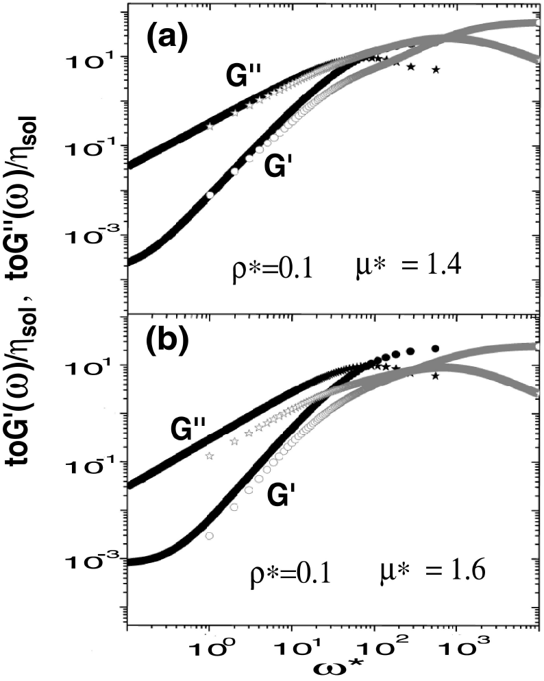
Figure 4. Logarithm of viscoelastic moduli versus frequency and two dipolar strength and fixed concentration. Theory for G' is denoted with symbol and simulation with . Theory result of G'' is denoted by gray open star and simulation by

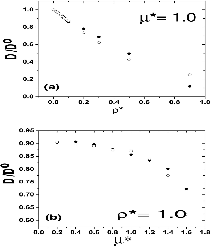
Figure 5. Translational self-diffusion coefficient D/D0 versus; density (a) and dipole strength (b). Simulation calculations are depicted with symbol and theory predictions with

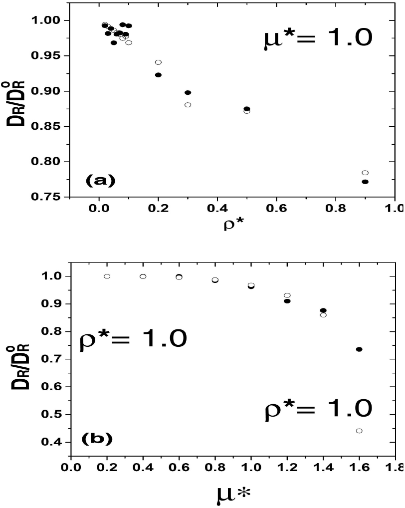
Figure 6. Rotational self-diffusion coefficient DR /DR0 versus; density (a) and dipole strength (b). Simulation calculations are depicted with symbol and theory predictions with

Whereas for the rotational diffusion DR/DR0=1/[1+ΔζRζ0R] and the friction contribution is

ΔζRζ0R=limω03πβd3G(ω)ω*=128πρ*μ*41050dxj1(x)2(6+x2)×67(τs,1*)2+38(τs,0*)2. (43)

G'' is given further by Eq. (45) below, j1(x) is the spherical Bessel function of order 1 and ζ0R=πd3ηsol.

In Figs. 5 and 6 simulation values are given by symbol whereas the theory calculations of diffusion coefficients are provided by symbol . From these plots, we can see that in general theory predictions for the diffusion properties yield good agreement with simulations both as a function of dipolar strength and ferrofluid concentration. The diffusion of the particles becomes restrained when there is an increase in dipolar interaction or concentration. We notice that the static translational and rotational self-diffusion coefficients are amenable to be measured experimentally. There are, however, independent Brownian dynamic simulation calculations for these properties reported in Refs.48,49.

5. Rotational diffusion microrheology

In this section, we provide the viscoelastic moduli of the ferrofluid when the probe particle performs rotational Brownian motion 7. From the friction function of Eq. (17) for the rotational diffusion of the probe particle we obtained the elastic modulus of the magnetic fluid

G'(ω)=(ω*3πβd3)16ρ*μ*4ω*1050dxj1(x)2×-67S,111(x)(τs,1*)21+(ω*τs,1*)2+38S,011(x)(τs,0*)21+(ω*τs,0*)2. (44)

And the viscous modulus is

G(ω)=(ω*3πβd3)128πρ*μ*41050dxj1(x)2(x2+1)×67(τs,1*)21+(ω*τs,1*)2+38(τs,0*)21+(ω*τs,0*)2. (45)

We propose to use our Eqs. (35-37) and (41) for the rheology of ferrofluids in an experimental study as follows: Ferro-particles need to be made with a fluorescence dye in order they do not absorb all light in experiments of video microscopy which allows determining their positions. At low concentration and a proper selection of wavelength as indicated in Ref. 4 may allow for this case. Since the measurement of each particle orientation would be difficult, even with the determination of the spatial coordinates, it is feasible to obtain the radially symmetric component g(r) of the pair correlation function using Eqs. (38) moreover, (39). Thus, it can be ignored the transversal contributions mnl = 110, 112. We have observed that for very low or very high concentrations the dipolar dependent terms are much smaller either in the viscoelastic moduli of Eqs. (35,37) , Eq. (41), and in the diffusion coefficients, Eqs. (42-43), then their symmetric parts which depend on h000. The resulting expressions will still depend only on the radially symmetric S,000 component, and yet they will provide a good approximation for these properties.

6. Conclusions

Using a Langevin equation approach we derived analytical expressions for the elastic G' and loss modulus G'' valid in linear viscoelasticity of a ferrofluid and no external magnetic fields. We approximated the collective dynamic of fluctuation in concentration regarding a single relaxation time. Such temporal decay of thermal fluctuations coincides with a Maxwell model of viscoelasticity. These expressions depend on the microstructure of the magnetic fluid through the structure factor determined by direct particle interactions. For model systems at different thermodynamic states of equilibrium, magnetic moment and concentration, the prediction of the viscoelasticity yields the observed trends that result from Langevin dynamic calculations. At low frequencies of thermal fluctuations of polarization, the dissipative mode is dominant. At high frequencies, the ferrofluid behaves as an elastic material. The viscous modulus at long times relates to the self-diffusion coefficient of translational and rotational diffusion of a ferro-particle. We point out that the approach presented in our manuscript allows the determination of three essential dynamical properties of the magnetic suspension: the viscosity, translational and rotational tracer diffusion coefficients. Both diffusion coefficients display the same tendency as the results of simulation calculations. In a forthcoming manuscript, we introduce our extension of the present approach to include time-dependent external magnetic and electric fields acting on ferrofluids in the regime of applied linear stationary shear flows and its comparison with existing experiments.

Acknowledgments

The authors acknowledge to the General Coordination of Information and Communications Technologies (CGSTIC) at CINVESTAV for providing HPC resources on the Hybrid Supercomputer ”Xiuhcoatl” that have contributed to the research results reported within this paper.

References

1. S. Odenbach, Colloidal Magnetic Fluids, 1st Edition (2009), Springer, Berlin. [ Links ]

2. S. Odenbach, Magnetoviscous Effects in Ferrofluids, 1st Edition (2002), Springer, Berlin . [ Links ]

3. M. Gert-Noritzch, D.Y. Borin and S. Odenbach, J. Phys.: Condens. Matter 23 (2011) 346002. [ Links ]

4. A. Mertelj, A. Rešetič, S Gyergyek, D Makovec and M. Čopič, Soft Matter 7 (2011) 125. [ Links ]

5. T.G. Mason and D.A. Weitz, Phys. Rev. Lett., 74 (1995) 1250. [ Links ]

6. B. Yendeti B, G. Thirupathi, A. Vudaygiri and R. Singh R, Eur. Phys. J. E, 37 (2014) 70. [ Links ]

7. Z. Chen and T.G. Mason , Phys. Rev. Lett. , 90 (2003) 018304. [ Links ]

8. R. Colin, M. Yan, L. Chevry, J.F. Berret, and B. Abou, EPL, 97 (2012) 30008. [ Links ]

9. H.W. Müller and M. Liu, Ferrofluids (Lecture Notes in Physics vol 594) 1st Edition (2002), ed S Odenbach, Springer, Berlin . [ Links ]

10. H. Pleiner, M. Liu and H.R. Brand, Rheol. Acta. 37 (2004) 502. [ Links ]

11. H.W. Müller and M. Liu , Phys. Rev. E, 64 (2001) 061405. [ Links ]

12. M.I. Shliomis, Sov. Phys. JETP, 34 (1972) 1291. [ Links ]

13. M.I. Shliomis, J. Magn. Magn. Mater., 159 (1996) 236. [ Links ]

14. M.I. Shliomis, Phys. Rev. E , 64 (2001) 063501. [ Links ]

15. Y.L. Raikher and M.I. Shliomis, Adv. Chem. Phys., 87 (1994) 595. [ Links ]

16. P. Ilg, E. Coquelle and S. Hess, J. Phys.: Condens. Matter , 18 (2006) S2757. [ Links ]

17. P. Ilg P and S. Hess , Z. Naturforsch., 58a (2003) 589. [ Links ]

18. A.Y. Zubarev, J. Fleischer andS. Odenbach , Physica A, 358 (2005) 475. [ Links ]

19. A.Y. Zubarev , Physica A , 392 (2013) 72. [ Links ]

20. J. Claracq, J. Sarrazin and J.P. Montfort, Rheol. Acta. , 43 (2004) 38. [ Links ]

21. A. Jordan, R. Scholz, K. Maier-Hauff, M. Johannsen and P. Wust, J. Magn. Magn. Mater. , 225 (2001) 413. [ Links ]

22. R. Hernández, A. Sarafian, D. López and C. Mijangos, Polymer, 46 (2004) 5543. [ Links ]

23. Y.L. Raikher and V.V. Rusakov, JETP, 83 (1996) 988. [ Links ]

24. H. Yamaguchi, X.D. Niu, X.J. Ye, M. Li and Y. Iwamoto, J. Magn. Magn. Mater. , 324 (2012) 3238. [ Links ]

25. A. Leschhorn A, J.P. Embs and M. Lücke, J. Phys.: Condens. Matter , 18 (2006) S2633. [ Links ]

26. J.P. Embs , B. Huke, A. Leschhorn andM. Lücke , Z. Phys. Chem., 222 (2008) 527. [ Links ]

27. M.A. Martens, R.J. Deissler, Y. Wu, L. Bauer, Z. Yao, R. Brown and M. Griswold, Med. Phys., 40 (2013) 022303. [ Links ]

28. Z. Wang and C. Holm, Phys. Rev. E , 68 (2003) 041401. [ Links ]

29. S. Mahle S , P. Ilg and M. Liu , Phys. Rev. E , 77 (2008) 016305. [ Links ]

30. O. Müller, D. Hahn and M. Liu , J. Phys.: Condens. Matter , 18 (2006) S2623. [ Links ]

31. H. Atkuri, G. Cook, D.R. Evans, C.I. Cheon, A. Glushchenko, V. Reshetnyak, Y. Resnikov, J. West and K. Zhang, J. Opt. A: Pure Appl. Opt., 11 (2009) 024006. [ Links ]

32. S.H.L. Klapp, J. Phys.: Condens. Matter , 17 (2005) R525. [ Links ]

33. F. Li, O. Buchnev, C.I. Cheon , A. Glushchenko , V. Reshetnyak , Y. Resnikov , T.J. Sluckin and J.L. West, Phys. Rev. Lett. , 97 (2006) 147801. [ Links ]

34. T.M. Squires and T.G. Mason , Annu. Rev. Fluid Mech., 42 (2010) 413. [ Links ]

35. R.J. DePuit and T.M. Squires, J. Phys.: Condens. Matter , 24 (2012) 464106. [ Links ]

36. M. Hernández-Contreras and H. Ruiz-Estrada, Phys. Rev. E , 68 (2003) 031202. [ Links ]

37. J. Keizer, Statistical Thermodynamics of Nonequilibrium Processes, 1st Edition (1987), Springer-Verlag, New York. [ Links ]

38. J.P. Hansen and I.R. McDonald I R, The theory of Simple Liquids, (London: Academic Press, 1980) [ Links ]

39. M. Hernández-Contreras , M. Medina-Noyola and O. Alarcón-Waess, Chem. Phys. Lett., 256 (1996) 483. [ Links ]

40. J.C. Bacri, R. Perzynski, D. Salin and J. Servais, J. Phys. (Paris), 48 (1987) 1385. [ Links ]

41. J.C. Bacri , A. Cebers, A. Bourdon, G. Demouchy, B.M. Heegaard, B. Kashevsky and R. Perzynski , Phys. Rev. E , 52 (1995) 3936. [ Links ]

42. P.H. Fries and G.N. Patey, J. Chem. Phys., 82 (1985) 429. [ Links ]

43. G. Nägele, M. Medina-Noyola , R. Klein and J.L. Arauz-Lara, Physica 149A, (1988) 123. [ Links ]

44. S. Plimpton, J. Comput. Phys., 117 (1995) 1. [ Links ]

45. R. Colin, L. Chevry , J.F. Berret and B. Abou , Soft Matter , 10 (2014) 1167. [ Links ]

46. B.U. Felderhof and R.B. Jones, Phys. Rev. E , 48 (1993) 1084. [ Links ]

47. B. Bagchi B and A. Chandra, Phys. Rev. Lett. , 64 (1990) 455. [ Links ]

48. P. Ilg and M. Kröger, Phys. Rev. E , 72 (2005) 031504. [ Links ]

49. A. Sreekumari A andP. Ilg , Phys. Rev. E 88 (2013) 042315. [ Links ]

Received: October 03, 2017; Accepted: November 29, 2017

Creative Commons License This is an open-access article distributed under the terms of the Creative Commons Attribution License