INTRODUCTION

In terms of catch volume, shark fishing in the southern Gulf of Mexico, both multi-specific and artisanal, is the 10^th most important in Mexico. According to ^{Rodríguez-De la Cruz et al. (1996)} and ^{Martínez-Cruz et al. (2016)}, the sharpnose shark Rhizoprionodon terraenovae (Richardson 1836), is one of the main exemplars of dominant shark species in the commercial catch (45.9%), in terms of weight (^{SEMARNAT, 2000}).

The sharpnose shark is a particular coastal species that is adapted to tropical water and its adult length ranges from 29 cm to 110 cm. This shark has a viviparous development and a gestation length estimated at 11 or 12 months, bearing between five and twelve pups (^{Castillo-Géniz, 1992}). As a result of these characteristics, this shark is considered a k-type strategist, implying that its capacity to respond to environmental variations -such as changes in human activities, especially overfishing- is quite limited (^{Hoenig & Gruber, 1990}). For this reason, the review of oscillations in its capture may provide insight to the potential influence of different environmental variables on this shark’s landing volumes behavior. Among the environmental variables that could affect the abundance of sharks, primary production fluctuations caused by solar radiation oscillations related to solar activity are among the main ones (^{Lluch-Cota, 2004}). Therefore, the joint analysis of time series for landings of R. terraenovae and solar activity cycles may allow the identification of possible coincidences when subjected to an innovative approach that we discuss below. Similar exercises have been carried out for other fisheries in Mexico, such as the Gulf of California sardines -where evidence showed a dominant frequency of about 5 years (^{Huato-Soberanis & Lluch-Belda, 1987})- but have never been applied before to the R. terraenovae fishery in the southern Gulf of Mexico. This type of analysis may be an important contribution and baseline for the construction of future predictive models.

The effect of solar activity -as determined by the number of sunspots- on the biosphere, on fluctuations of the Earth’s magnetism, temperature, radiance intensity, and energy fluxes, has already been tested. Several studies have related fish catch with solar cycles. Helland-Hanses and Nansen, quoted by ^{Hjort (1914)}, conducted one similar pioneer analysis and provided evidence on an existing relationship between water temperature, currents, and their effects on fishing activities resulting from solar activity. Likewise, the study conducted by ^{Bulatov (1995)} in the Bering Sea is one of the most comprehensive studies on this subject, consisting of a historical review of fishing activity according to spawning, demographic structure, size, cohort composition, and particular conditions of the pollock Theragra chalcogramma (Pallas, 1814) stocks. In his research, ^{Bulatov (1995)} concluded that the largest classes were constituted during the ascendant phase of the Wolf’s cycle curve. Harmonics of 11 years in catch volumes of salmon Coregonus lavaretus (Linnaeus, 1758), perch (Perca fluviatilis Linnaeus, 1758), and cyprinids Rutilus rutilus (Linnaeus, 1758) were detected in Lake Constance, Canada, and provided evidence about an existing relationship. This was determined by an indirect tie with cyclical conditions from environmental variables, which were accordingly related to solar activity and striking over such populations’ biological stages (^{Hartmann, 1995}). A cyclical variation of scallop recruitment was estimated in southern Australia, associated to corresponding harmonics of the west wind blowing in that region (^{Thresher, 1994}). Oscillations in solar activity are responsible for climatic fluctuations in a scale ranging from 40 to 60 years and are related to variations on abundance of diverse commercial fisheries in Russia (^{Davydov, 1986}). Similarly, ^{Guisande et al. (2004)} proved that abundance of sardine Sardina pilchardus (Walbaum, 1792) in the Iberian Atlantic is governed by solar activity. ^{Vanselow and Ricklefs (2005)} demonstrated the existence of a relationship between solar activity and stranded sperm whales Physeter macrocephalus Linnaeus, 1758, in the North Sea.

Time series analysis is a research technique that was developed many years ago. Its application to biological research has been limited, due to the inherent difficulty in gathering a data series of sufficient length. Thus, even though there is ample recognition of space and time oscillations of biological and ecological processes, and the fact that they respond to oscillatory forcing of high and low frequencies -such as diel variation, among the former and Earth translation, El Niño events, the North Atlantic Oscillation and sunspot cycles, for the latter- its application to the analysis of biological systems behavior has not really been fully exploited (^{Platt & Denman, 1975}).

Consequently, this study aims to analyze the possible relation between solar activity and the landing behavior of the sharpnose R. terraenovae along the Mexican shoreline of the southern Gulf of Mexico between 1940 and 2006.

MATERIALS AND METHODS

Registries of the annual volumes of catches of Rhizoprionodon terraenovae were reported as fresh weight landed on the different harbors of the southern Gulf of Mexico, as listed by the Governmental Statistical Yearbooks from 1940 to 2006 (^{SEMARNAP, 1940-2006}; Fig. 1). Annual averages of sunspot numbers (Zürich Index) were obtained from Solar-Geophysical Data Comprehensive Reports of ^{NOAA (2007)} at the following web address: https://www.ngdc.noaa.gov/stp/Solar/ftpsunspotnumber, and plotted on Figure 2.

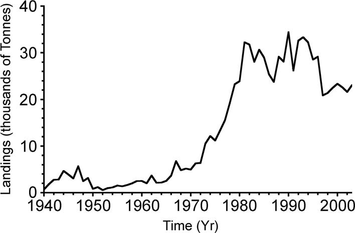
Figure 1 Time series (Yr) of sharpnose (Rhizoprionodon terraenovae) landings (thousands of tons) in the Gulf of Mexico between 1940 and 2003. There has been a strong increase in landings since the late 60s. 

Figure 2 Time series (Yr) of the average number of sunspots per year (Zürich Index) between 1749 and 2003. 

Processing the shark landings. The literature dealing with Catch per Unit Effort (CPUE) has approached the problem of splitting the original data into their different temporal components in several ways: linear methods, sine function, and spectral analysis. For the jumbo squid (Dosidicus gigas d’Orbigny [in 1834-1847], 1835), monthly catch data from 2002 to 2005 were grouped into three large zones, and the trend of the time series was removed by using a LOESS smoother. The residuals between the original and the LOESS trend curve were computed and analyzed using autocorrelation and cross-correlation at different lags, and a trigonometric model was fitted to detect seasonal oscillation (^{Zúñiga et al., 2008}). As for the sailfish fisheries in the Mexican Pacific, time series methods (the removal of two harmonics from their original CPUE data) were used to estimate CPUE trends as an abundance indicator (^{Macías-Zamora et al., 1994}).

If a survey is conducted in a time series looking for periods of around 11 years, high frequency events far from the target period must be eliminated (^{Emery & Thomson, 2004}). In the special case of shark-landing time series, due to a growing trend in fishing activities through time (Fig. 1), a very low frequency wave (1/64 Yr) with high energy was generated. Thus, in order to detect 11-year periodicity, a method must be applied in a way that eliminates the fishing -activity trend.

To eliminate this low frequency trend, we implemented the following procedure: a) A centered smooth (moving) average was computed for the shark-landing time series (L_n-2 + L_n-1 + L + L_n+1 + L_n+2)/5, where L is the landing in the nth time. b) By the least-squares method, a best-fit polynomial was computed for the smoothed series with a FORTRAN program prepared according to ^{Lawson and Hanson (1974)}. The resultant polynomial was:

CompLand(t) = 5x10^-05 t⁶ 0.0085 t⁵ + 0.4981 t⁴ 11.504 t³ + 91.268 t² 45.349 t + 1759 eq. 1

where CompLand(t) is the computed landing at time t. c) The polynomial was used to compute the landings as a function of time, as seen in Figure 3. d) From CompLand(t) and ObsLand(t) a catch-difference (anomaly) time series was generated (Dif(t), (Fig. 4). The differences time series (Dif(t)) was standardized. The procedure was as follows.

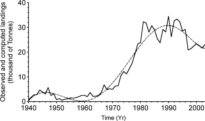
Figure 3 Time series (Yr) of sharpnose (Rhizoprionodon terraenovae) landings (thousands of tons) black line, and computed landings from the least-squares polynomial (dashed line). Differences between the two series were used for spectrum computations. 

Figure 4 Z standardized values of the difference between the observed landings and the polynomial computed data (z-landings). Z is defined as (x’ x_i)/σ, where x’ is the average, x_i the i-th landing difference data, and σ the standard deviation. 

The polynomial was computed from the smoothed landing time series, as stated above, while the differences were computed according the following equation:

Dif(t) = ObsLand(t) CompLand(t) eq. 2

where ObsLand(t) is the observed landing at time t, and CompLand(t) is the shark landing at time t computed from the polynomial. As usual in time series, analysis data were standardized (^{Bendat & Piersol, 1986}) by using z(t) values defined as follows:

z(t) = (Dif(t) Dif ’) / Stadev eq. 3

where z(t) is the normalized value at time t, Dif(t) is the difference obtained from the landings and the polynomial computed from eq. 2, and Dif’ and Stadev were the average and standard deviation of the Dif(t) time series. The z(t) time series was detrended as explained bellow.

The standardized difference time series of sharpnose landings (z(t)) and Zürich Index were studied through a spectral analysis, using two distinctive methods: Fast Fourier Transform (FFT, ^{Bendat & Piersol, 1986}) and Maximum Entropy (ME, ^{Calmet et al., 1984}). FFT is a model coherent in the definition of energy density, but has the disadvantage that the number of data needed has to be cut down to a power of 2 (~2^6,8). Through the ME method a good frequency resolution might be obtained, but energy densities and spurious frequencies may suffer from alterations when the number of used poles (m) is not properly computed (^{Calmet et al., 1984}).

Data used for the analysis of shark catches came from a series of 67 years, where the series trend was removed. The time series was competed to 2⁸. The time series obtained through this technique was analyzed afterwards in order to obtain specific spectral figures.

The trend was removed from the sunspot time series, although it was not necessary to append it up recursively as the data came from ~ 307 years. The most common technique for trend removal is to fit a straight-line equation using econometric tools such as least-squares procedures. The linear regression takes the form of a straight line with an intercept of b₀ and a slope b₁, which is subtracted from the original data values {x_n} (^{Bendat & Piersol, 1986}). That is, if x₁’ is the new value without the trend, then

{x₁’}={x₁} {1 b₁+ b₀},

{x₂’}={x₂} {2 b₁+ b₀}, . . .

{x_n’}={x_n} {n b₁ + b₀}

The new time series so obtained were detrended and the requisite of stationarity for the FFT method accomplished (^{Brigham, 1974}).

The processes of energy transference between the sun and the biosphere are not registered immediately by the latter. The reason is that, in general, there is a lag between a general stimulus and its response; thus, the potential correlation between both would not be statistically significant if an immediate response was supposed. If an appropriate delay is considered -that is to say, if the correlation is estimated for a response displayed 1, 2,.., n intervals later- linear correlations become statistically significant.

In order to determine the delay between R. terraenovae landings and solar activity, a cross-correlation analysis was computed, using the differences series (z(t)) and Sspot(t). Through this technique, the level of likeliness between both variables was not only visible -defining the independent variable as “fixed” and the dependent variable as “lagged”-, but the delay time between both processes could be observed as well (^{Legendre & Legendre, 1979}).

Briefly, removal of a trend through a polynomial of shark landings was applied. Time series of shark landings and sunspots were detrended. Spectral analyses were applied with the FFT and ME techniques in an effort to add the advantages of the implementation of both methods. Different authors have performed a similar analysis to the same data set and obtained a frequency of 10.6 years for the Zürich Index (^{Vanselow & Ricklefs, 2005}).

RESULTS

Original time series of data from R. terraenovae landings (Fig. 1) and solar activity (R_z) (Fig. 2) are presented. R. terraenovae landings show a clear trend to increase with time, which reflects an increase in fishing activities. Thus, in order to detect any cyclical behavior, for both series the trend was removed through the polynomial (Fig. 3).

Normalized values (z(t)) of the differences between the observed sharpnose shark (R. terraenovae) landings (ObsLand(t)) and the computed landings through the polynomial (ComLand(t)) are observed in Figure 4. The series, thus transformed and normalized, is referred to as sharpnose shark time series in the text that follows and should not be confused with the sharpnose-shark landings series.

The power spectra of the sharpnose shark time series, through the joint examination using both methods (ME and FFT), are shown on Figure 5. The resulting spectrum of shark landings showed other peaks of higher frequency. The most striking feature detected in the shark spectrum is that the major oscillation energy reached a frequency of 2.51 x 10^-9 Hz (the peak of 12.8 years), (Fig. 5).

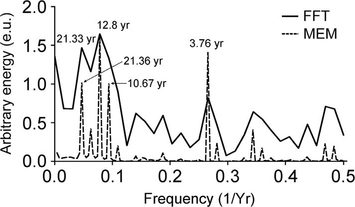
Figure 5 Power spectrum by the Maximum Entropy Method (MEM; m= 60 poles) of the z-landings time series (dashed line), and by the Fast Fourier Transform method (FFT), (solid line). Conspicuous frequencies are noted with their equivalent period in years. 

Different peaks of lower frequency can be identified as well (Fig. 5). It is likely that the peak around 22 years is, up to where we can analyze the series, the second one of major energy, although the sharpnose shark landings series is not large enough to provide absolute certainty.

Figure 6 shows the power spectrum of the average number of solar spots (Zürich Index) time series. The main harmonic detected for ME analysis is a sharp peak of 10.88 years. For FFT analysis two peaks are present: 11.1 years and 10.66 years. Note that the data of the yearly average of sunspot numbers resulted in a neat peak for both spectra, for that obtained by ME, as well as by FFT (Fig. 6).

Figure 6 Power spectrum by the Maximum Entropy Method (MEM; m= 40 poles) of the average number of sunspots (Zürich Index) time series (dashed line), and by the Fast Fourier Transform method (FFT), (solid line). The well-defined sunspot frequency is noted with its equivalent period in years. 

Cross-correlation reveals a delay between the average number of solar spots and sharpnose-shark landings (Fig. 7). A good correlation was obtained when sharpnose-shark landings were delayed one year (R= 0.65) and two years (R= 0.60); further delay times had lower R’s.

Figure 7 Linear cross-correlation coefficients of z-landing time series versus the average number of sunspots (Zürich Index) time series. Each bar corresponds to a forward lag of one year of the z-landings. 

DISCUSSION

In time-series analysis, a common practice along the scientific community is the use of the complementary FFT and ME methods (^{Calmet et al., 1984}). Time series are useful to describe the potential environmental variations related to catch volumes of fish populations susceptible to exploitation (^{Ottersen et al., 1994}). The variation of catch volumes along different fishing stocks in distinctive parts of the world responds to periodical climatic variations of temperature, rainfall, cloud coverage, and evaporation, which interact with water temperature, salinity, density, and, consequently, water mass dynamics (^{Francis & Sibley, 1991}; ^{Mountain & Murawski, 1992}; ^{Ohtani & Azumaya, 1995}; ^{Studenetsky, 1995}; ^{Yang et al., 1995}).

By building a polynomial, we were able to obtain a time series amenable for use in spectral analysis. Without this adjustment, the increase in catch per fishing activity would have complicated the analysis, due to the great wave or harmonic introduced by fishing activity, which started during the late 60s and finished until the late 90s.

In coastal regions inhabited by R. terraenovae, several variables exert a marked influence in environmental fluctuations. The first and main one is temperature: Its positive anomalies coincide with a wider access of solar irradiance unleashing changes in wind intensity throughout tropical latitudes that, overall, modify humidity and, thus, cloud coverage. While the ocean surface stores an important amount of heat, the sea surface temperature (SST) reacts directly to solar forcing, even though a lag occurs. Related to what was described before, ^{Van Loon and Labitzque (1994)} detected that the reaction scale under which the process of energy exchange operates -coming from irradiance inputs- with the consequential thermal increment of the SST in tropical latitudesis year-to-year and responds to the same frequency of Wolf’s solar cycle.

A complete understanding of the behavioral dynamics of one or more communities would involve their study for several decades, in order to determine the underlying mechanisms that jeopardize fluctuations in the populations resulting from the perennial search for system equilibrium, which is periodically broken and in different time scales as a result of the climate’s influence.

Ocean-atmospheric variables, such as rainfall and water temperature -including their “modifiers”- are connected to solar activity cycles (^{Sánchez-Santillán, 1999}). The relationship occurs in such a way that, if organisms have a narrow relationship with the respective environmental variables and the latter have a periodical nature (^{Haig, 2003}; ^{Haig et al., 2005}), the same periodical pattern would be attained for the organisms’ behavior.

In this study, the analysis of a short shark-landing time series -with data from 66 years- was possible with the combined aid of two spectral methods (the ME and FFT methods).

The analyzed landing volumes of the sharpnose shark R. appeared because of a periodical behavior that coincided with Wolf’s solar activity cycle of 10.6 years.