1.Introduction
Nowadays, Free-Space-Optical (FSO) communication links are used for short distances
in the Local Area Network or Metropolitan Area Network. They are also being used for
long-distance links, particularly for conventional satellite and quantum security
applications 1-3. However, the process of designing
optical links in the classical and quantum domain requires, in addition to the
traditional optical power budget, to take into account diverse phenomena that affect
the overall performance, such as the atmospheric turbulence 4. The atmospheric turbulence modifies the refractive
index of air masses depending on the pressure and temperature value in such a way
that the optical field’s diverse parameters may be affected by this phenomenon.
Among these parameters are its phase, amplitude, state of polarization, orbital
angular momentum, and also some phenomena such as the quantum entanglement 5,6. In general, the FSO link is designed and
characterized, firstly, in the laboratory environment, then, a real implementation
at different distances is needed for different applications 7,8. However, the characterization of such links still
lacks a rigorous prior analysis regarding atmospheric turbulence. Although there are
some experimental proposals for atmospheric turbulence chambers, they present
important limitations and trade-offs such as 1) static or sometimes dynamic design
with reduced configuration parameters, 2) reduced limit of emulated link distances,
and 3) reduced control of atmospheric turbulence levels, among others 9,10. Several mathematical algorithms simulate the
effects of atmospheric turbulence over an optical field 11-14. However, to the best of our knowledge, such
algorithms do not determine the actual received optical power (measured in Watts)
for the different possible regimes of atmospheric turbulence based on
characteristics of physical devices. This document presents a technique for the
design and statistical evaluation of FSO links based on the simulation of the
optical information signal affected by different atmospheric turbulence levels. For
this purpose, we generate by simulation a data time series with a Gamma-Gamma
probability density function that allows modeling optical turbulence from low to
high turbulence regimes. We organized our paper as follows: Section 2 presents some
theoretical aspects of atmospheric turbulence and its effect over the optical power
and the spatial phase of the received signal. Section 3 presents the results
obtained in our simulations. Finally, Sec. 4 presents the conclusion and important
aspects of future work.
2.Theoretical background
2.1.Atmospheric turbulence theory
A parameter commonly used to indicate the level of atmospheric turbulence is the
scintillation index σI2 related to the irradiance of the optical field traveling through the
free space channel. But as the optical power and the irradiance are related, one
instead may use the power scintillation index σP2 for a particular distance link (L) using Eq. (1):
σP2=⟨PRx2(L)⟩⟨PRx(L)⟩2-1,
(1)
where PRx(L) denotes the optical power affected by turbulence at a distance L(m)
from the optical transmitter, ⟨⟩ is the ensemble average (sample mean), and, the log power variance
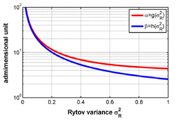
(Rytov variance) σR2 is related to σP2 as σP2=exp(σR2)-1, considering that σP2≈σR2 for σR2≪1, i.e., applicable for weak turbulence regime, as
Fig. 1 shows. Thus, the σR2 value is described for long-distance links (i.e.,
for plane wavefront) as Eq. (2) 15:
σP2=σR2=1.23Cn2k7/6L11/6.
(2)
On the other hand, for spherical wavefront, σP2=0.4σR2=0.5Cn2k7/6L11/6. Here, Cn2(m-2/3) is the index of refraction structure parameter, k=2π/λ is the optical wavenumber (m), λ is the wavelength, and L(m) is the
propagation path length between transmitter and receiver systems. Also, Cn2 may be considered constant for a given condition of optical
turbulence in horizontal links. However, if the weather conditions change, the
value of Cn2 will change accordingly 15. We will see this effect more clearly in vertical
links where the Cn2 value will depend on each atmospheric layer through which the
optical beam travels. In our paper, we calculate the Cn2 value considering only the transmitter and receiver locations in a
horizontal link for a fixed condition of optical turbulence
(i.e., we defined the full effect of the turbulence through
the atmosphere as a black box).
As Eq. (1) showed, σP2 parameter depends on the receiver optical power PRx(L) affected by the stochastic variations of the optical turbulence in
addition to diverse (static) losses introduced by the free-space optical
channel. As Eq. (1) showed, σP2 parameter depends on the receiver optical power PRx(L) according to the free space loss (Ls)
(i.e. Free-Space Path Loss law is shown in Eq. (3)).
Although other kinds of losses are present in an FSO link
(e.g., beam divergence, weather conditions, pointing) and
laws, as Beer’s law. Hence, PRx=PTxLs
16.
Ls=λ4πL2
(3)
The stochastic behavior of atmospheric optical turbulence is commonly described
using a lognormal probability density function (pdf) due to its relative
simplicity. However, this description is valid just for low to medium turbulence
values. On the other hand, there are other more complex probability density
functions, such as the called Gamma-Gamma, whose results are valid for weak to
strong turbulence levels. The Gamma-Gamma (f
GG) pdf describes turbulence as a function of small and large-scale
variations. Equation (4) shows the relation of f
GG with PRx with α and β parameters being the effective number of small-scale
and large-scale eddies of the scattering environment, respectively 16. Commonly, Eq. (4) is related
to the irradiance (W/m2), but considering the active area
(m2) of a suitable photodetector, Eq. (4) can be expressed using
the optical power received.
fGG(PRx;α,β)∝2αβa+β2ΓαΓβ×PRxα+β2-1kα-β(2αβPRx)
(4)
where Γ(⋅) is Gamma function, and Ka(⋅) is the modified Bessel function of second kind of order α. The
parameters of the Gamma-Gamma function are related to the Rytov variance using
Eqs. (5) and (6) under the assumption of plane wave and negligible inner scale,
which corresponds to long propagation distance and small detector area 17.
α=gσR=exp0.49σR21+1.11σR12/57/6-1-1
(5)
β=hσR=exp0.51σR21+1.69σR12/55/6-1-1
(6)
For instance, if σR2=0.3 implies the values of α = 8.42 and β = 6.91. Figure 2 shows the behavior of g(σR) and h(σR) for the range 0<σR2≤1, from weak to strong turbulence regimes.
2.2.Data affected by simulated atmospheric turbulence
To simulate the temporal behavior of the optical channel, we generate a
time-series for the data-signal affected by different atmospheric turbulence
levels that satisfy a Gamma-Gamma distribution based on 18. Also, in our simulations, we take into
account the static attenuation on the optical field when it travels through the
free space optical channel according to Beer-Lambert law, which is described as τ(λ,L), where τ is the transmittance or atmospheric transmission. In
particular, two stochastic processes are used to describe the small-scale and
large-scale turbulence, which are described by the Gamma functions, Γ(α) and
Γ(β), respectively. Therefore, xk+1(α) and yk+1(β) describe the temporal data (i.e., an ensemble of
many particular values, k) that satisfies the functions Γ(α) and Γ(β)from Eqs.
(7) and (8) 18.
xk+1α=xkτc+∆t+∆t(ξk2-1)2α+2xkτcΔtα1/2ξk1+Δt
(7)
yk+1β=ykτc+∆t+∆t(ξk2-1)2β+2ykτcΔtβ1/2ξk1+Δt
(8)
Here, ξk is a normal uncorrelated White Gaussian Noise (WGN) process,
τc is the correlation time between samples, Δt is the sampling
time, and k is the particular sample. In this way, in Eqs. (7) and (8) are used
to calculate the normalized received optical power, PRx¯(α) and PRx¯(β), respectively, as shown in Eqs. (9) and (10). Since the stochastic
processes described in Equations (7) and (8) are independent, the multiplication
of both processes generates a time-series signal that satisfies a Gamma-Gamma
distribution, PRx¯(α,β) , which is also normalized as Eq. (10) shows.
PRx¯(α)∝xk+1(α), PRx¯(β)∝yk+1(β),
(9)
PRx¯(α,β)∝xk+1(α)yk+1(β).
(10)
Finally, the optical signal received affected by simulated atmospheric
turbulence, as well as the attenuation introduced by free space, is described in
Eq. (11), where Prx is the denormalized form of the complete expression at the right
side of Eq. (11).
Prx=PTxτ(λ,L)PRx¯(α,β).
(11)
It is convenient to note that Eq. (11) is the optical power received affected
only by the turbulence and optical channel attenuation according to Beer-Lambert
law. However, in a real-world environment, it is required to take also into
account the photodetector responsivity R [A/W], so Eq. (11) is modified as:
YRx=R[PTxτ(λ,L)PRx¯(α,β)⊗h+z],
(12)
where YRx is the photocurrent at the receiver, h is the impulse response of an
ideal low-pass filter representing the limited bandwidth of photoreceiver, and z
is any front-end noise in the photoreception stage (e,g., thermal, among others)
19. All the parameters are
time-dependent, except R. For coherent detection schemes used in quantum communication links,
the Standard Quantum Limit (SQL) imposes that 𝑧 is determined by shot
noise.
2.3.Phase fluctuation induced by atmospheric turbulence
Another essential aspect to consider in FSO links is the phase fluctuation in a
spatial region of the detector. The atmospheric turbulence modifies the phase of
the signal in different regions of the wavefront that can affect the
communications link’s performance, particularly for coherent detection schemes.
There are various phase drifts in an FSO link (e.g., optical phase drift caused
by phase noise); however, we will only consider spatial phase fluctuation
because the other phase noises are not caused by turbulence. It is possible to
determine the power spectrum of these phase fluctuations using Eq. (13),
representing a thin phase screen 20-22.
φn(K)=0.033Cn2k2Lx-11/3=0.033r0-5/3K-11/3,
(13)
where K is the transverse coordinate, considering that a single atmospheric layer
(multiple atmospheric layers simulation requires a high-end computer system)
based on the aperture diameter DG of the telescope used.
r0 is the wavefront coherence diameter describing the spatial
correlation of phase fluctuations in the receiver plane due to random
inhomogeneities in the atmosphere’s refractive index. In our case, r0=(k2Cn2L)-3/5, and it is constant because we consider just a single atmospheric
layer. In particular, the phase screen does not modify the amplitude; in fact,
the optical phase is the only parameter affected. It is important to mention
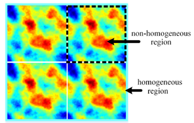
that Eq. (13) is based on Discrete Fourier Transform (DFT), which means that the
phase screen is periodic. This argument imposes a wrong hypothetical scenario of
small non- homogeneous regions inside a homogeneous large region (see Fig. 3) that have to be considered for large
region analysis taking into account DG and r0
parameters.
2.4.Mean Signal to Noise Ratio for atmospheric turbulence link
Evaluating the performance of an FSO link affected by atmospheric turbulence are
used parameters such as the electrical Signal-to-Noise Ratio (SNR) and the Bit
Error Rate (BER) at the output of the photoreceiver for different modulation
schemes. Equation (14) shows the SNR without taking into account the atmospheric
turbulence, where h is the Planck’s constant v = c/ λ, and B is the bandwidth of
the photoreceiver used 21.
Also, Eq. (14) is only considering the SQL; in another way, the thermal noise
has to be considered.
SNR0=is2σN2=⟨YRx2⟩σN2∝PTxτ(λ,L2hvB .
(14)
However, since the optical power received is affected by dynamical and random
atmospheric turbulence, it is not possible to calculate the SNR for specific
power received. Therefore, the mean SNR (E[SNR]) measurement is required, as Eq. (15) shows 21:
ESNR=SNR0PTxτ(λ,L)PTxτ(λ,L)PRx-(α,β)+σP2(DG)SNR02
(15)
2 where σP2(DG) is the power variance in the plane of the detector, DG is
the aperture diameter of the receiver (i.e., first lens of the telescope). In
the same way, σP2(DG)=σP2(0,L+Lf), where L
f
is the focal length. In particular, σP2(DG)=0 means that atmospheric effects are not present in the link. Also, σP2 can be related to σI2 (flux irradiance variance). In particular, if the terms, PTxτ(λ,L) and ⟨PTxτ(λ,L)PRx¯(α,β)⟩ are considered with same mean values, then:
PTxτ(λ,L)PTxτ(λ,L)PRx-(α,β)=1
(16)
Therefore, the Eq. (15) can be rewritten as Eq. (17) shows, which is related to
Eqs. (5-6)
ESNR=SNR01+σP2(DG)SNR02=SNR01+expσP2-1(DG)SNR02
(17)
On the other hand, E[SNR] can also be related to the phase perturbations
described by Eq. (13). In particular, calculating the Cn2 (based on a particular atmospheric turbulence level), it is possible
to determine the σR2 value and, next, determine the α and β parameters by Eqs. (5-6).
Finally, in order to calculate the mean Bit Error Rate ( E[BER]) for OOK modulation and Direct Detection (DD), it is necessary to
normalize the received power using x=Prx/⟨Prx⟩ in Eq. (18). Here, p(x) is the Gamma- Gamma probability density
function that represents the atmospheric turbulence for different levels 21.
EBER=12∫0∞p(x)erfcESNRX22dx≈12∑i=1∞p(xi)erfcESNRxi22
(18)
In particular, Eq. (18) is presented as a continuous integration of the power
received affected by atmospheric turbulence, however; it is possible to modify
the mathematical expression to optimize the computational simulation based on
narrow bins (i) that represent certain optical power measured.
3.Results and analysis
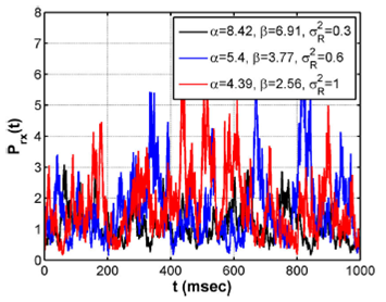
In order to determine the temporal behavior of a hypothetical optical signal
received, some technical settings were established, such as PTx=500 mW, L = 10,000 m, λ = 1550 nm, τc = 20 ms, 5 x 10⁵
samples with Δt=10-4s and bit rate at 350 KHz. All parameters are variable in the simulation,
and, in fact, some parameters are simplified or normalized to show general results.
Figure 4 shows the optical signal on the
receiver side based on Eqs. (3) and (11) for different turbulence regimes. Besides,
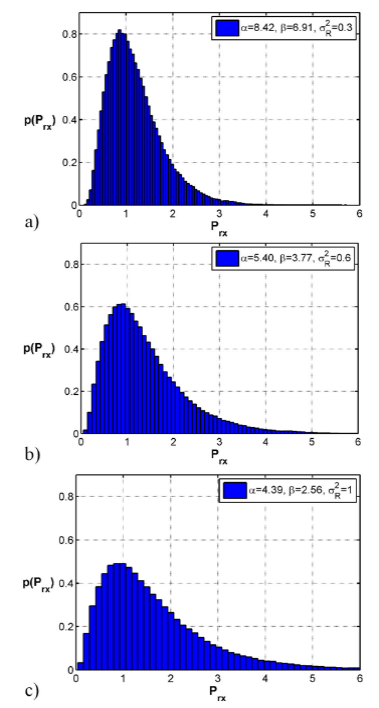
Fig. 5 shows the distribution of numerical
data of the optical signal received considering weak, moderate, and strong
atmospheric turbulence regime with particular values for σR2, α, and β. These distributions have a Gamma-Gamma probability density
function shape. In particular, Cn2=2.22×10⁻¹⁶ m-2/3 for σR2=0.3, and Cn2 can be calculated for a particular turbulence regime. Thus, the results
showed in Figs. 4 and 5 can be modified according to atmospheric turbulence levels
(i.e., modifying Cn2 parameter) based on the Rytov variance and Gamma-Gamma parameters.
Figure 5 shows the distribution of the samples
and, regarding the strong turbulence regime, the mean value of PRx is less than the other regimes because PRx presents more fluctuations in the samples ensemble, i.e., the optical
power received is increased for those samples that had less optical power in the
weak and moderate turbulence regimes.
Thus, for a strong turbulence regime, the probability is increased for all samples
that represent high power received (PRx>2), and decreased for PRx=1. On the other hand, Fig. 6 shows
the probability density function considering a fixed ensemble data related to Δt=10 ms in order to visualize the particular behavior of the optical signal
related to the temporal variation using a turbulence level condition close to the
moderate turbulence regimes. It can be seen that the density function does not
change; that is, it remains Gaussian, so it can be interpreted that the optical
state has not changed due to the non-linearity of the atmospheric channel.
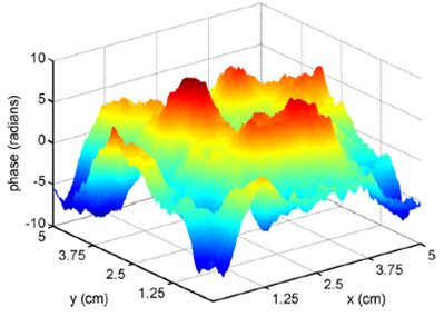
Figure 7 shows the simulated phase screen
considering the parameters mentioned and an aperture diameter DG = 5 cm
based on Eq. (13). The results show that the phase screen imposes a phase variation
added to the phase noise of the optical signal for a particular spatial position on
the receiver side. The maximum and minimum variations are 8 and -8 radians,
respectively, for Cn2=2.22×10⁻¹⁶ m-2/3 (i.e., meaning a moderate turbulence level, although
this parameter can be modified). In order to clarify, the maximum and minimum
variations do not imply generalized phase changes; in fact, the mean phase variation
is less than 0.5 radians. It is important to clarify that the phase screen showed is
a random numerical result according to (13), i.e., in general, different
representations of phase screen can be generated maintaining the maximum and minimum
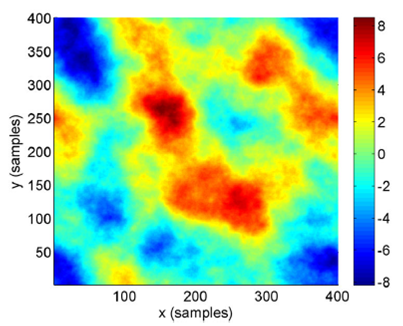
phase variation similar. Also, Fig. 7 is
represented using the physical dimension of the receiver aperture diameter, while
Fig. 8 shows the same results in a
different representation considering the spatial samples based on the sample
resolution, i.e., 400 samples for x and y-axis, which means that 1 sample is
equivalent to 0.0125 cm. This resolution is optimal in order to characterize small
and large eddies present in the turbulence medium.
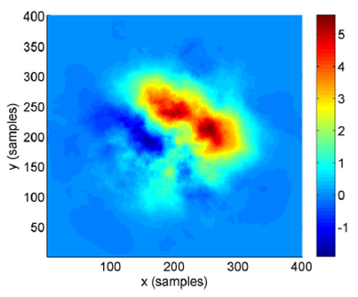
Therefore, considering a Gaussian beam transmitted through the atmospheric turbulence
and a single-phase screen, both represented before, it is possible to obtain a
spatial phase representation as Fig. 9 shows.
It is important to mention that the results can vary because they are evaluated
based on random variables. Nevertheless, the results generated are very useful for
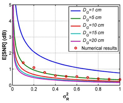
FSO communication systems. Besides Fig. 10
shows the theoretical and numerical results for the mean SNR parameter considering
different atmospheric turbulence levels (from weak to strong turbulence) and
aperture diameters. In particular, the σP2 values for each simulated series-time showed in Fig. 4 are affected by different DG values, as Eq.
(17) showed. Therefore, the mean SNR is reduced for stronger atmospheric turbulence
levels, i.e., 1.4 dB for σR2=0.33 and 0.36 dB for σR2=1. The latter, due to the increasing variation of the values generated and
showed in Fig. 5. Besides it is important to
mention that the mean SNR is also increased based on the aperture diameter. Hence,
the atmospheric turbulence characterization in an FSO link has to be performed based
on a particular and well-known photodetector and passive optical devices. The SNR0
value was considered constant (i.e., 10 dB), which is related to Eq. (14).
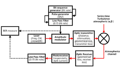
Figure 11 shows the block diagram used in
order to obtain the simulation results considering particular values for the
different subsystems of the overall communication system. The simulation was
performed using a homologated Matlab script based on the VPI photonics program,
although the OptiSystem program is also useful. In particular, a bit sequence
generator at 350 Kbps (related to τc = 20 ms) is used, a pulse generator
based on Non-return-to-zero (NRZ) and Low Pass Filter (fc=0.7×bit rate) produces the input digital signal to the amplitude modulator. Concerning
the optical source, a CW laser (500 mW) at λ =1550 nm (v = 193.41 THz) and Δv = 1
MHz is used. Thus, the electrical input signal modulates the optical signal. Next,
the simulation considers some features of the optical transmitter, such as distance
link (10 Km), attenuation (2.3 dB/Km), geometrical losses (10 dB), and transmitter
losses (3 dB). The photoreceiver has a responsivity of 1 A/W and a dark current of
10 nA. Regarding the atmospheric channel, a multiplying point permits the
introduction of the series-time turbulence based on Gamma-Gamma distribution
function.
Finally, Fig. 12 shows the results of E[BER] for different E[SNR] values based on Fig. 11. Remember
that according to Eq. (17), the mean SNR value depends on some parameters such as
DG, σR2, and SNR0. In this case, DG = 5 cm, σR2=1, and SNR0 are modified in relation to particular
photodetectors. However, it is possible to use a particular photodetector and vary
the Rytov variance, i.e., a particular mean SNR value can mean a combination of
different parameter values presented in the free space link and receiver scheme. In
fact, the results simulated based on series-time data affected by atmospheric
turbulence described for Gamma-Gamma function are closely related to the theoretical
results showed in 21.
4.Conclusions
The accurate characterization of the optical signal transmitted through the
atmospheric channel is necessary in order to offline research the possible effects
in a future hypothetical FSO link to improve the overall performance. Thus,
simulated series-time signals affected by atmospheric turbulence were generated
based on two stochastic processes described by a Gamma probability density function
in order to calculate the performance of a particular FSO link. The simulation
permits to visualize an optical signal affected by different atmospheric turbulence
regimes, i.e., from σR2=0.1 to σR2=1, and calculate the mean SNR and mean BER using a time-interval of 1
second. The simulation can be expanded to large time-intervals according to the
performance parameters required (e.g., Bit Error Rate), transmission rates used in
particular FSO links, and scheme modulations (e.g., Quadrature Amplitude Modulation
(QAM), Phase Shift Keying (PSK), among others). Also, the spatial phase was
simulated for particular σR2 value, although it is possible to modify the atmospheric condition
parameters to determine the correct spatial phase perturbation. In particular, the
correlation time value used is directly obtained based on the temporal covariance
function for a particular condition of the FSO link, i.e., the time value for 1/e of
the normalized temporal covariance function is the correlation time. This condition
is described based on the distance of link, Rytov variance, and the transverse wind
speed for Taylor’s frozen-turbulence hypothesis 21. This means that the simulation proposed is suitable
to analyze only the FSO links that satisfy the conditions mentioned. Finally, the
numerical results regarding the mean SNR and mean BER for different atmospheric
turbulence regimes are highly related to the theoretical performance. In fact, if
this simulation proposal is used for the design and proof of concept of FSO links
previous to the real implementation, it is necessary to provide technical details of
each optical and optoelectronic device to increase the accuracy of the numerical
results.


 nueva página del texto (beta)
 Inglés (pdf)
 Artículo en XML
 Referencias del artículo
 Enviar artículo por email
 Citado por SciELO
  Similares en
SciELO
Similares en
SciELO 
 Permalink