Appendix

Equations of the CGE model

The first step is to incorporate the intermediate goods and the composite good as part of the analysis. The composite good is obtained by aggregating the capital and labour through the production function of the composite good, which is a Cobb–Douglas form function (Equation 2). Thus, this problem is related with the production of the composite good that will be used as input for the gross domestic output. This can be realised as follows:

Subject to:

That is, the profit–maximisation problems for the j–th firm subject to the composite goods where:

: profit of the j–th firm producing composite factor Y_j
Y_j: composite factor used by the j–th firm
F_h,j: the h–th factor used by the j–th firm
X_i,j: intermediate input of the i–th good used by the j–th firm
: price of the j–th composite factor
: price of the h–th factor
β_h,j: share coefficient in the composite factor production function (exogenous)
b_j: scaling coefficient in the composite factor production function (exogenous)

And we have in addition the factor requirements of the firm,

the intermediate inputs requirements, which depend directly on the volume of production Z_j,

the composite factor used by the j–th firm as function of the output,

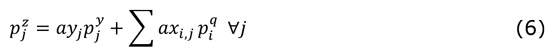
where ax_i,j: input requirement coefficient of the i–th intermediate input for a unit output of the j–th good (exogenous) and ay_j the input requirement coefficient of the j–th composite good for a unit output of the j–th good (exogenous); and finally, the price of the j–th gross domestic output or unitary cost of production

where is the price of the i–th composite good.

In the second place, it is necessary introduce the government into the model. The public sector is important by the following reasons: first, the influence through the taxes on income and prices; second, the government expenditure plays a crucial role in the economy consumption; and finally, the trade tariffs are considered.

The next equations are the taxes system, in which, is assumed that the government levied the household income at a fixed tax rate (Equation 7), an ad valorem tax on output (Equation 8) and an ad valorem import tariff on international trade (Equation 9)

where:

T^d: direct tax (exogenous)
: production tax on the j–th good (exogenous
: import tariff on the i–th good (exogenous)
: direct tax rate
: production tax rate on the j–th good (exogenous)
: import tariff rate on the i–th good (exogenous)
FF_h: endowments of the h–th factor for the household (exogenous)
M_i: imports of the i–th good
: government consumption of the i–th good
: price of the i–th imported good

The following equation is the government expenditure equation which assumes that all the taxes revenues are spent in consumption, which means that there is no public deficit. This expenditure is realised in fixed ratios between each of the goods:

Where μ_i is the share of the i–th good in government expenditure (exogenous).

The investment and saving are considered as follow. The household savings and the government fiscal balance can be defined in terms of its average propensities to save:

where:

S^p: household savings
S^g: government savings
ss^p: average propensity for savings by the household (exogenous)
ss^g: average propensity for savings by the government (exogenous)

The relation between investment and savings is defined by the economic identity I=S, thus the investment derives from the savings of households and government plus the current account balance,

where:

: demand for the i–th investment good
S^f: current account deficits in foreign currency terms (exogenous)
ε: foreign exchange rate
λ_i: expenditure share of the i–th good in total investment (exogenous)

Since the recent addition of the government and investment and savings inside the model, some previous equations need to be modified. Thus, the new household and government demands functions are:

The last important characteristic of this standard CGE model is the presence of the external sector, this extension makes possible to switch from a closed model to an open one. Therefore, is assumed that the export and import prices quoted in foreign currency terms are exogenous, that is, a small country without enough market shares to be able to influence in the world prices:

where: and are the export and import prices, both in terms of foreign currency and exogenous, and is the export price in terms of domestic currency.

Additionally, the Balance of Payments is assumed in equilibrium, where E_i are the exports of the i–th good.

Since the standard CGE model includes the consumption both domestic and imported goods, we have to assume that exist difference between good produced in the domestic economy and the ones that are imported. At this point, we use Armington's assumption. The Armington composite goods have a nested consumption structure, since assumes that the imported goods are not consumed or used directly. Instead of this, the composite good comprises imports and the corresponding domestic goods, whose proportions are determined by the elasticity of substitution. The Armington composite good is defined as follow:

where:

D_i: the i–th domestic good
Q_i: the i–th Armington composite good
γⁱ: scaling coefficient in the Armington composite good production funcion (exogenous)
δm_i, δd_i: input share coefficients in the Armington composite good production function (exogenous)
η_i: parameter defined by the elasticity of substitution (exogenous) (ηi =(σi − 1)/σi, ηi ≤ 1)
σi: elasticity of substitution in the Armington composite good production function and the demand functions for imports and the domestic good:

The last point on international trade is to split the production process between imported and domestic goods. This production is described by a constant elasticity of transformation (CET) function, where, according on the relative price between exports and domestic goods, the supply for each of these markets changes:

where:

Z_i: gross domestic output of the i–th good
: production tax rate on the i–th gross domestic output (exogenous)
θ_i: scaling coefficient of the i–th transformation (exogenous)
ξe_i, ξd_i: share coefficients for the i–th good transformation (exogenous)
Φ_i: parameter defined by the elasticity of transformation (exogenous)

Finally, impose the market–clearing conditions to assure the equilibrium in all the markets. The first equation is for the Armington composite goods and the second one is the factor market–clearing condition:

Equation 24 is the factor market–clearing condition, that is, total demand for h–th factor by firms must be equal to total endowments of h–th factor, assumed to be given in the economy.